Ensemble Methods for Machine Learning Outline Motivations and

Ensemble Methods for Machine Learning

Outline • Motivations and techniques – Bias, variance: bagging – Combining learners vs choosing between them: • bucket of models • stacking & blending – Pac-learning theory: boosting • Relation of boosting to other learning methods—optimization, SVMs, …

WHY BIAS AND VARIANCE MOTIVATE ENSEMBLES

Bias and variance • For regression, we can decompose the error of the learned regression into two terms: bias and variance – Bias: the class of models can’t fit the data. – Fix: a more expressive model class. – Variance: the class of models could fit the data, but doesn’t because it’s hard to fit. – Fix: a less expressive model class.

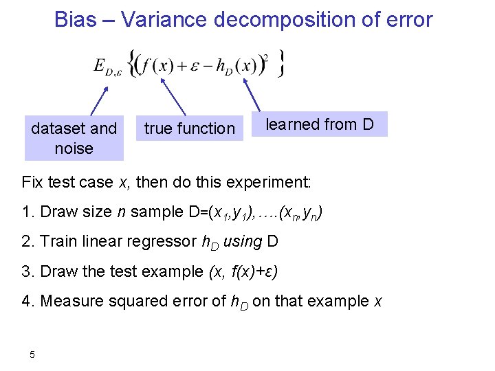
Bias – Variance decomposition of error dataset and noise true function learned from D Fix test case x, then do this experiment: 1. Draw size n sample D=(x 1, y 1), …. (xn, yn) 2. Train linear regressor h. D using D 3. Draw the test example (x, f(x)+ε) 4. Measure squared error of h. D on that example x 5

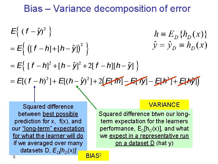
Bias – Variance decomposition of error Squared difference between best possible prediction for x, f(x), and our “long-term” expectation for what the learner will do if we averaged over many datasets D, ED[h. D(x)] 6 VARIANCE Squared difference btwn our longterm expectation for the learners performance, ED[h. D(x)], and what we expect in a representative run on a dataset D (hat y) BIAS 2

Bias-variance decomposition • This is something real that you can (approximately) measure experimentally – if you have synthetic data, or a large dataset • Different learners and model classes have different tradeoffs – large bias/small variance: few features, highly regularized, highly pruned decision trees, … – small bias/high variance: many features, less regularization, unpruned trees, …

Bias and variance Domingos, A Unified Bias-Variance Decomposition and its Applications, ICML 2000 • For classification, we can also decompose the error of a learned classifier into two terms: bias and variance – Bias: the class of models can’t fit the data. – Fix: a more expressive model class. – Variance: the class of models could fit the data, but doesn’t because it’s hard to fit. – Fix: a less expressive model class. • How else can we reduce variance?

Bias and variance • Beside tradeoffs: How can we reduce variance? – If we want to reduce standard error (~sd/sqrt(n)) of a sample what can we do? – Get more samples! • Here the experiment is a dataset D and a classifier h. D – Can we get more “samples” of the experiment? – Idea 1: randomize the algorithm somehow and run it many times – Idea 2: randomize the dataset somehow….

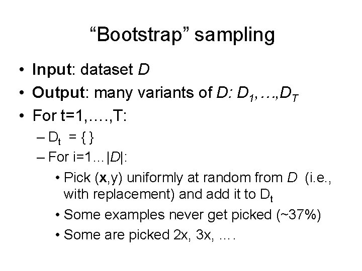
“Bootstrap” sampling • Input: dataset D • Output: many variants of D: D 1, …, DT • For t=1, …. , T: – Dt = { } – For i=1…|D|: • Pick (x, y) uniformly at random from D (i. e. , with replacement) and add it to Dt • Some examples never get picked (~37%) • Some are picked 2 x, 3 x, ….

Bootstrap Aggregation (Bagging) • Use the bootstrap to create T variants of D • Learn a classifier from each variant • Vote the learned classifiers to predict on a test example

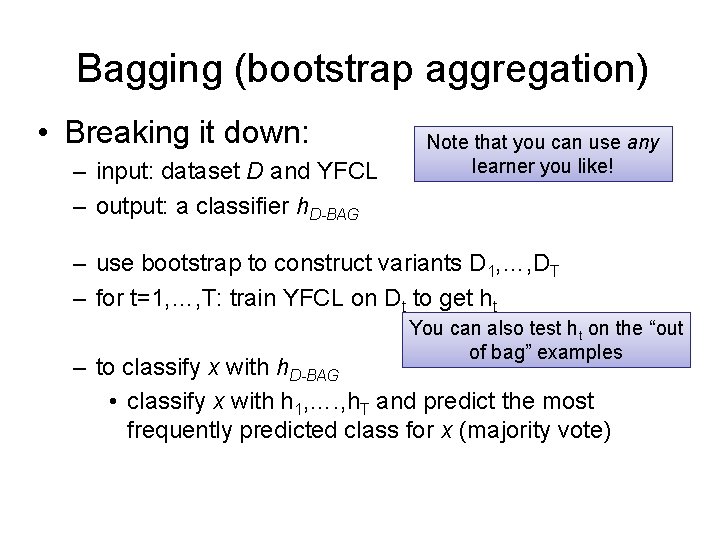
Bagging (bootstrap aggregation) • Breaking it down: – input: dataset D and YFCL – output: a classifier h. D-BAG Note that you can use any learner you like! – use bootstrap to construct variants D 1, …, DT – for t=1, …, T: train YFCL on Dt to get ht You can also test ht on the “out of bag” examples – to classify x with h. D-BAG • classify x with h 1, …. , h. T and predict the most frequently predicted class for x (majority vote)

Bagging (bootstrap aggregation) • �Experimentally: – even with pruning, decision trees have low bias but high variance. – bagging usually improves performance for decision trees and similar methods – it doesn’t help for certain other methods (e. g. , nearest neighbor) which have low variance – It reduces variance without increasing the bias.

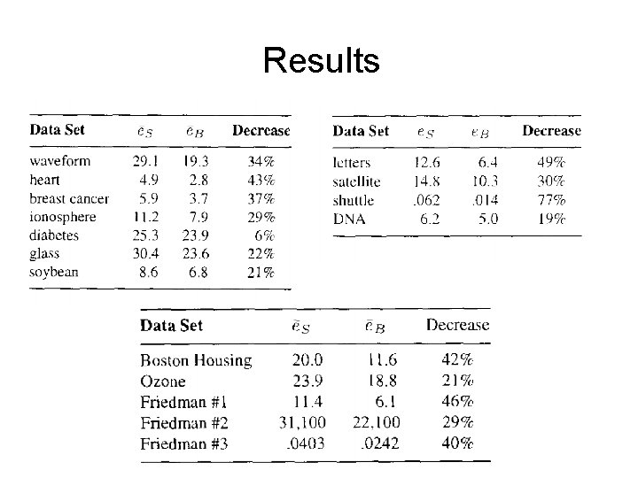
Results

COMBINING VERSUS CHOOSING BETWEEN CLASSIFIERS

Scenario 1 • You’re the chief scientist at the hot new startup, nothingbutfrogs. com • Kleiner-Perkins just gave your new company $20 M in funding… – …but you need to stay ahead of the competition! – …you hire Kevin’s sister, brother, and six of his first cousins and put them to work! – Each tries a different learner and you pick the best one…or can you do better?

Scenario 2 • You’re building a new classifier learner for class • The professor just gave the class tens of thousands of dollars of grant money for time on Amazon’s EC 2 cluster – …does that help you?

COMBINING MULTIPLE LEARNERS (OR MULTIPLE PEOPLE’S WORK ON BUILDING/TUNING LEARNERS)

Simplest approach: A “bucket of models” • Input: – your top T favorite learners (or tunings) • L 1, …. , LT – A dataset D • Learning algorithm: – Use 10 -CV to estimate the error of L 1, …. , LT – Pick the best (lowest 10 -CV error) learner L* – Train L* on D and return its hypothesis h*

Pros and cons of a “bucket of models” • Pros: – Simple – Will give results not much worse than the best of the “base learners” • Cons: – What if there’s not a single best learner? • Other approaches: – Vote the hypotheses (how would you weight them? ) – Combine them some other way? – How about learning to combine the hypotheses?

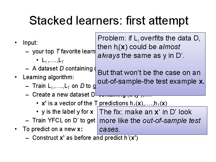
Stacked learners: first attempt Problem: if Li overfits the data D, • Input: then hi(x) could be almost – your top T favorite learners (or tunings) always the same as y in D’. • L 1, …. , LT – A dataset D containing (x, y), …. But that won’t be the case on an • Learning algorithm: out-of-sample-the test example x. – Train L 1, …. , LT on D to get h 1, …. , h. T – Create a new dataset D’ containing (x’, y’), …. • x’ is a vector of the T predictions h 1(x), …. , h. T(x) • y is the label y for x The fix: make an x’ in D’ look – Train YFCL on D’ to get h’more --- which the predictions! likecombines the out-of-sample test • To predict on a new x: cases. – Construct x’ as before and predict h’(x’)

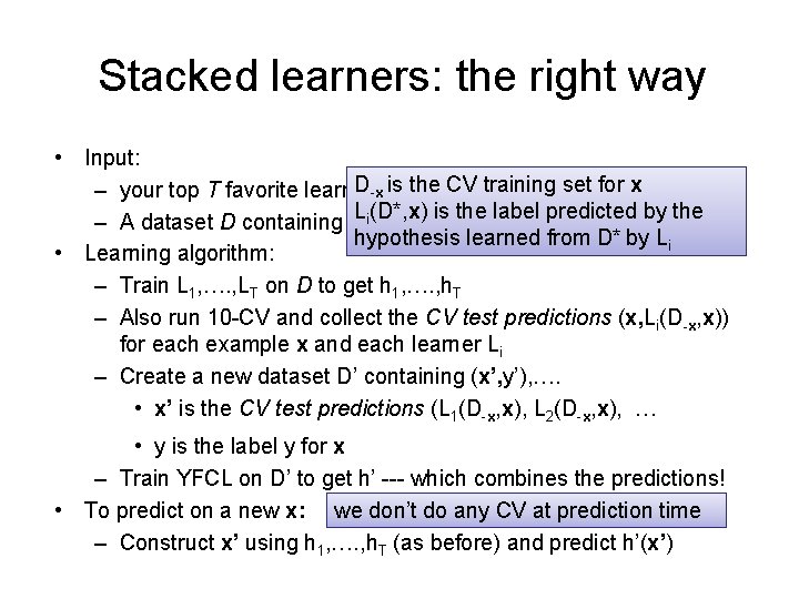
Stacked learners: the right way • Input: D-x is CV training set Tfor x – your top T favorite learners (orthe tunings): L 1, …. , L Li(D*, x) – A dataset D containing (x, y), …. is the label predicted by the hypothesis learned from D* by Li • Learning algorithm: – Train L 1, …. , LT on D to get h 1, …. , h. T – Also run 10 -CV and collect the CV test predictions (x, Li(D-x, x)) for each example x and each learner Li – Create a new dataset D’ containing (x’, y’), …. • x’ is the CV test predictions (L 1(D-x, x), L 2(D-x, x), … • y is the label y for x – Train YFCL on D’ to get h’ --- which combines the predictions! • To predict on a new x: we don’t do any CV at prediction time – Construct x’ using h 1, …. , h. T (as before) and predict h’(x’)

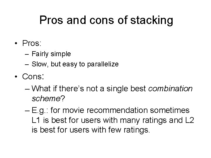
Pros and cons of stacking • Pros: – Fairly simple – Slow, but easy to parallelize • Cons: – What if there’s not a single best combination scheme? – E. g. : for movie recommendation sometimes L 1 is best for users with many ratings and L 2 is best for users with few ratings.

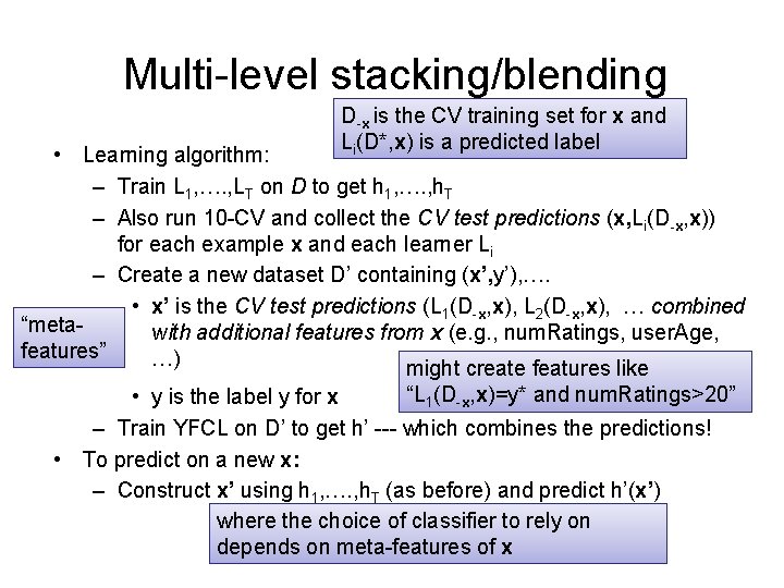
Multi-level stacking/blending D-x is the CV training set for x and Li(D*, x) is a predicted label • Learning algorithm: – Train L 1, …. , LT on D to get h 1, …. , h. T – Also run 10 -CV and collect the CV test predictions (x, Li(D-x, x)) for each example x and each learner Li – Create a new dataset D’ containing (x’, y’), …. • x’ is the CV test predictions (L 1(D-x, x), L 2(D-x, x), … combined “metawith additional features from x (e. g. , num. Ratings, user. Age, features” …) might create features like “L 1(D-x, x)=y* and num. Ratings>20” • y is the label y for x – Train YFCL on D’ to get h’ --- which combines the predictions! • To predict on a new x: – Construct x’ using h 1, …. , h. T (as before) and predict h’(x’) where the choice of classifier to rely on depends on meta-features of x

Comments • Ensembles based on blending/stacking were key approaches used in the netflix competition – Winning entries blended many types of classifiers • Ensembles based on stacking are the main architecture used in Watson – Not all of the base classifiers/rankers are learned, however; some are hand-programmed.

BOOSTING

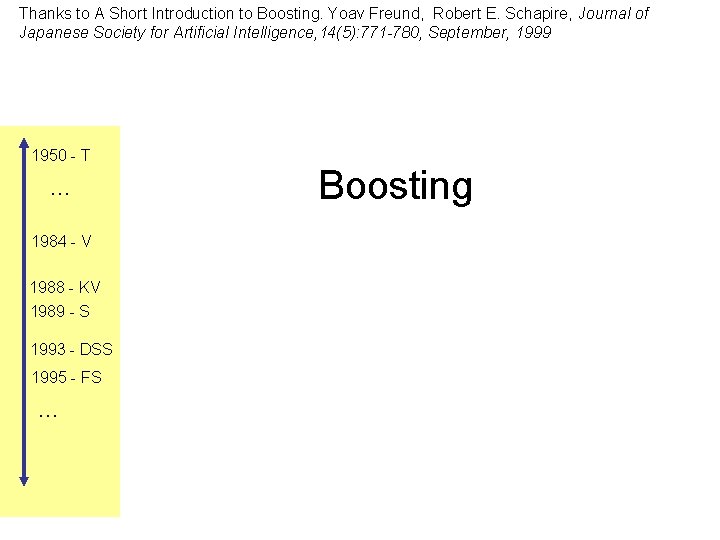
Thanks to A Short Introduction to Boosting. Yoav Freund, Robert E. Schapire, Journal of Japanese Society for Artificial Intelligence, 14(5): 771 -780, September, 1999 1950 - T … 1984 - V 1988 - KV 1989 - S 1993 - DSS 1995 - FS … Boosting

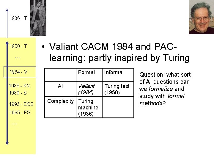
1936 - T 1950 - T … • Valiant CACM 1984 and PAClearning: partly inspired by Turing 1984 - V 1988 - KV 1989 - S 1993 - DSS 1995 - FS … AI Formal Informal Valiant (1984) Turing test (1950) Complexity Turing machine (1936) Question: what sort of AI questions can we formalize and study with formal methods?

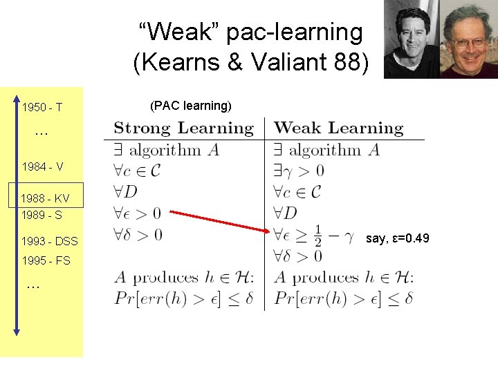
“Weak” pac-learning (Kearns & Valiant 88) 1950 - T (PAC learning) … 1984 - V 1988 - KV 1989 - S 1993 - DSS 1995 - FS … say, ε=0. 49

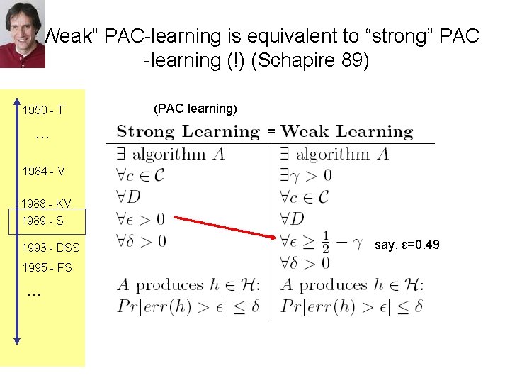
“Weak” PAC-learning is equivalent to “strong” PAC -learning (!) (Schapire 89) 1950 - T … (PAC learning) = 1984 - V 1988 - KV 1989 - S 1993 - DSS 1995 - FS … say, ε=0. 49

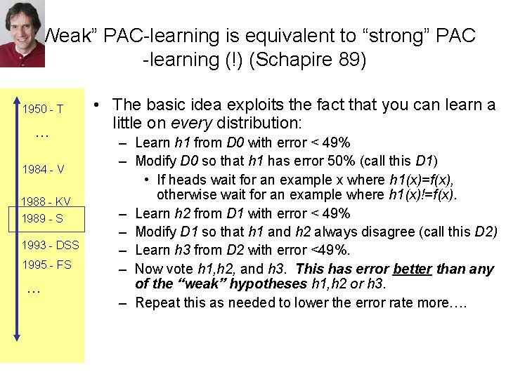
“Weak” PAC-learning is equivalent to “strong” PAC -learning (!) (Schapire 89) 1950 - T … 1984 - V 1988 - KV 1989 - S 1993 - DSS 1995 - FS … • The basic idea exploits the fact that you can learn a little on every distribution: – Learn h 1 from D 0 with error < 49% – Modify D 0 so that h 1 has error 50% (call this D 1) • If heads wait for an example x where h 1(x)=f(x), otherwise wait for an example where h 1(x)!=f(x). – Learn h 2 from D 1 with error < 49% – Modify D 1 so that h 1 and h 2 always disagree (call this D 2) – Learn h 3 from D 2 with error <49%. – Now vote h 1, h 2, and h 3. This has error better than any of the “weak” hypotheses h 1, h 2 or h 3. – Repeat this as needed to lower the error rate more….

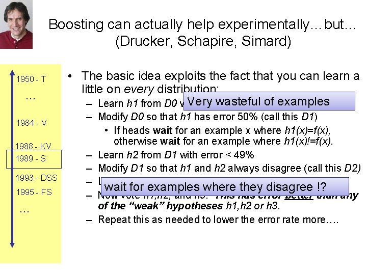
Boosting can actually help experimentally…but… (Drucker, Schapire, Simard) 1950 - T … 1984 - V 1988 - KV 1989 - S 1993 - DSS 1995 - FS … • The basic idea exploits the fact that you can learn a little on every distribution: Very wasteful – Learn h 1 from D 0 with error < 49% of examples – Modify D 0 so that h 1 has error 50% (call this D 1) • If heads wait for an example x where h 1(x)=f(x), otherwise wait for an example where h 1(x)!=f(x). – Learn h 2 from D 1 with error < 49% – Modify D 1 so that h 1 and h 2 always disagree (call this D 2) – Learn h 3 from D 2 with error <49%. wait for examples where they disagree !? – Now vote h 1, h 2, and h 3. This has error better than any of the “weak” hypotheses h 1, h 2 or h 3. – Repeat this as needed to lower the error rate more….

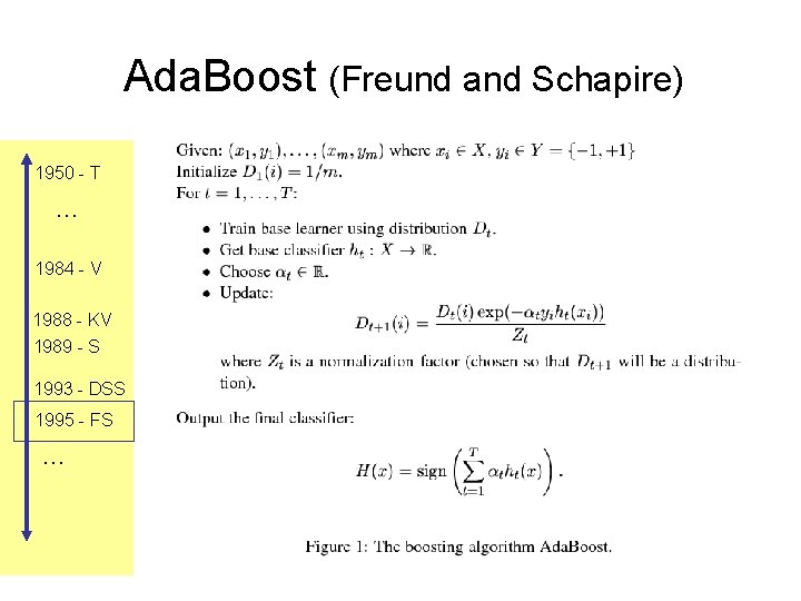
Ada. Boost (Freund and Schapire) 1950 - T … 1984 - V 1988 - KV 1989 - S 1993 - DSS 1995 - FS …

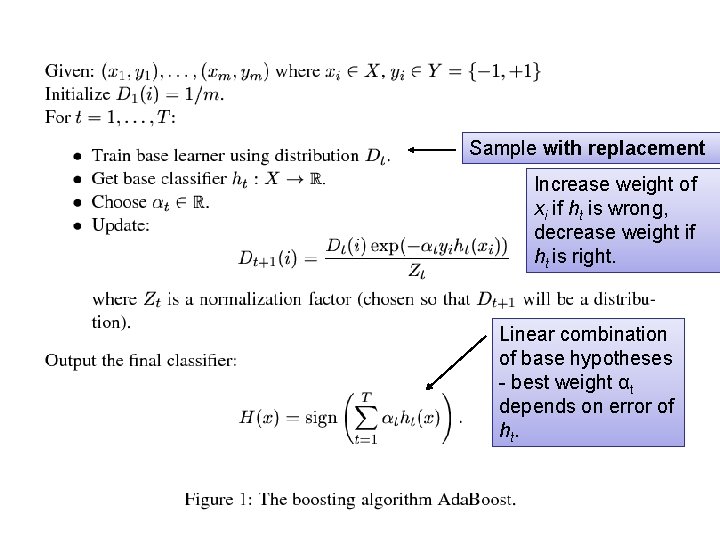
Sample with replacement Increase weight of xi if ht is wrong, decrease weight if ht is right. Linear combination of base hypotheses - best weight αt depends on error of ht.

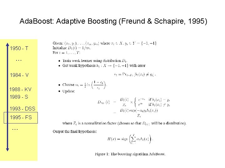
Ada. Boost: Adaptive Boosting (Freund & Schapire, 1995) 1950 - T … 1984 - V 1988 - KV 1989 - S 1993 - DSS 1995 - FS …

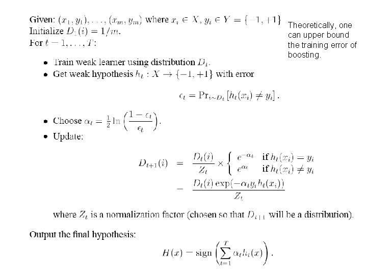
Theoretically, one can upper bound the training error of boosting.

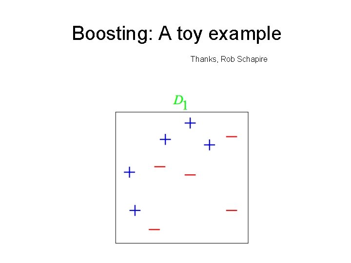
Boosting: A toy example Thanks, Rob Schapire

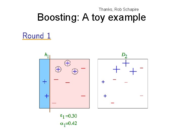
Thanks, Rob Schapire Boosting: A toy example

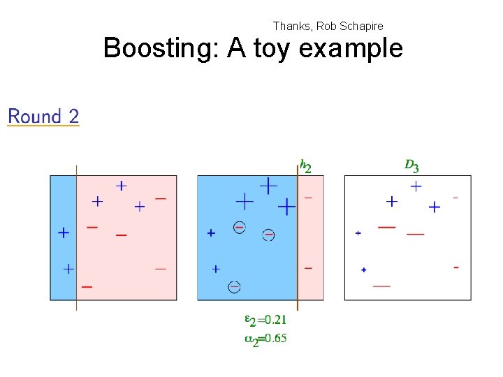
Thanks, Rob Schapire Boosting: A toy example

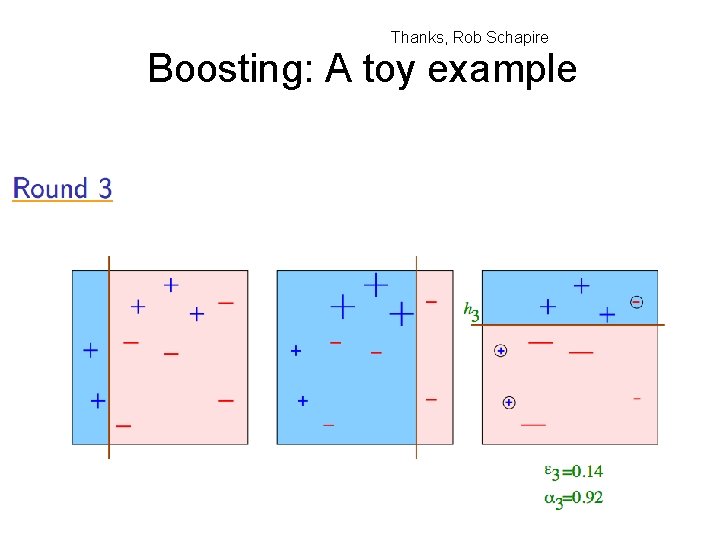
Thanks, Rob Schapire Boosting: A toy example

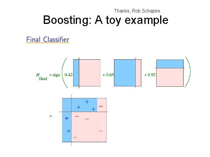
Thanks, Rob Schapire Boosting: A toy example

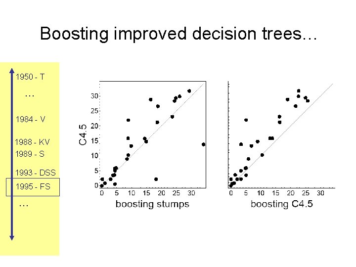
Boosting improved decision trees… 1950 - T … 1984 - V 1988 - KV 1989 - S 1993 - DSS 1995 - FS …

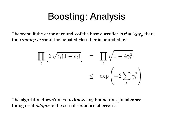
Boosting: Analysis Theorem: if the error at round t of the base classifier is εt = ½-γt, then the training error of the boosted classifier is bounded by The algorithm doesn’t need to know any bound on γt in advance though -- it adapts to the actual sequence of errors.