ENROLLMENT AND RETENTION FORECASTING USING MONTE CARLO METHOD

ENROLLMENT AND RETENTION FORECASTING USING ‘MONTE CARLO METHOD AIR Forum 2017 Rachel Link, University at Buffalo Michael Randall, University at Buffalo 1

Introduction to the University at Buffalo • • • Flagship university in the State University of New York System Member of the Association of American Universities Headcount: 20, 411 undergraduates; 9, 772 graduates (Fall 2016) ‘Degrees awarded: ~8, 700 annually More than 110 undergraduate and 300 graduate/professional programs 2

Challenge: Identifying Continuing UG Students Our enrollment model was created several years ago, and does not reflect changes in targets, leadership, and populations over time. ‘- Changing demographics and new institutional focus require a need to accurately predict what the continuing undergraduate population will be each semester. Focus on academic planning, space utilization, and course planning require accurate student counts in advance of semester start dates. 3

How can we accurately forecast the number of continuing students? • Due to changes in demographics, university practices, and degree programs, just using the averages of the last several years won’t work • How do we accurately predict continuing enrollments when there are so many factors that influence whether or not a ‘-particular student will re-enroll? • The answer: using a subset of predictive analytics called simulative analysis 4

What are simulative analytics? • Simulative analytics take the same patterns from the predictive analytics (which use equations to identify likely future results by using past patterns) and identify a range of future possibilities. ‘- • This range is then examined to see the likelihood of a specific result, rather than identifying one result alone • Simulative analytics is really a subset of predictive analytics: it also uses past results to identify potential future results 5

Introduction to Monte Carlo • The Monte Carlo Method uses repeated random sampling to generate simulated data to use with a mathematical model – we are accounting for risk in order to make decisions (in this case, planning for returning students) ‘- • This model is built from a statistical analysis: in our case, from the results from our binary logistic regression model • We build the regression equation and identify which variables are significant, and then run the simulations • Our results will yield the estimated values and display them in a histogram, showing the range of expected returning students 6

Coming Up with the Variables What factors might influence a student’s decision to return, and how could we collect those data? • • ‘- Quality factors (GPA, prior academic performance, SAP) Academic plan (major) Financial factors (Federal student loans, Pell eligibility) Length of time at the institution (total number of terms, continuous terms enrolled) • Behavior while at the institution (changing majors, resigning or withdrawing from courses) • Demographic factors (race/ethnicity, gender, age, citizenship) 7

Building the model Included: • All degree-seeking, state-funded undergraduate students (~55, 800 students) ‘- • Five years of data (Fall 2012, Fall 2013, Fall 2014, Fall 2015, Fall 2016), for a total of four models (2012 -13, 2013 -14, 2014 -15, 2015 -16) • Calculating a Fall to Fall perspective (what percent of the currently enrolled undergraduate students in Fall 2016 will return for Fall 2017? ) 8

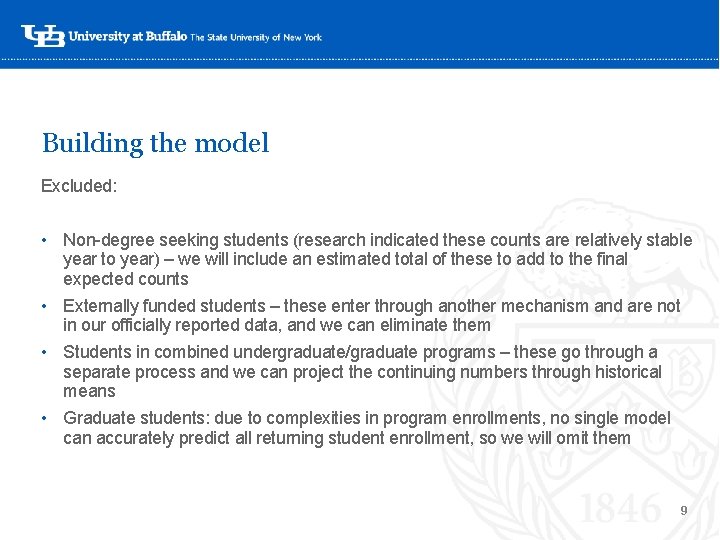
Building the model Excluded: • Non-degree seeking students (research indicated these counts are relatively stable year to year) – we will include an estimated total of these to add to the final ‘expected counts • Externally funded students – these enter through another mechanism and are not in our officially reported data, and we can eliminate them • Students in combined undergraduate/graduate programs – these go through a separate process and we can project the continuing numbers through historical means • Graduate students: due to complexities in program enrollments, no single model can accurately predict all returning student enrollment, so we will omit them 9

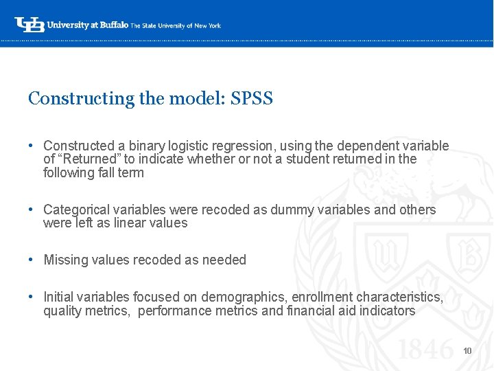
Constructing the model: SPSS • Constructed a binary logistic regression, using the dependent variable of “Returned” to indicate whether or not a student returned in the following fall term ‘- • Categorical variables were recoded as dummy variables and others were left as linear values • Missing values recoded as needed • Initial variables focused on demographics, enrollment characteristics, quality metrics, performance metrics and financial aid indicators 10

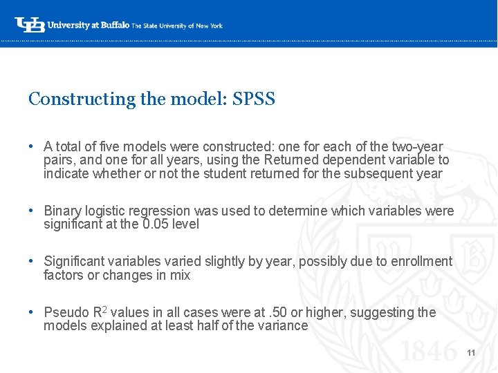
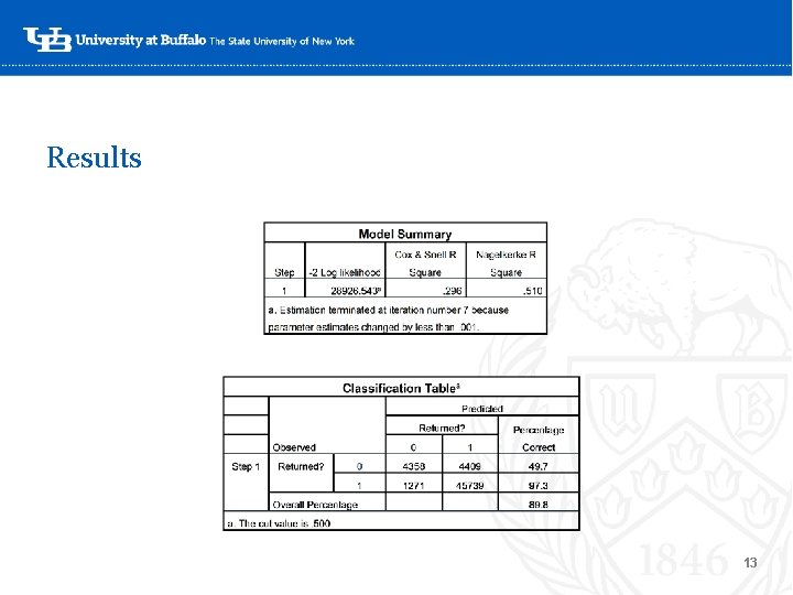
Constructing the model: SPSS • A total of five models were constructed: one for each of the two-year pairs, and one for all years, using the Returned dependent variable to indicate whether or not the student returned for the subsequent year ‘- • Binary logistic regression was used to determine which variables were significant at the 0. 05 level • Significant variables varied slightly by year, possibly due to enrollment factors or changes in mix • Pseudo R 2 values in all cases were at. 50 or higher, suggesting the models explained at least half of the variance 11

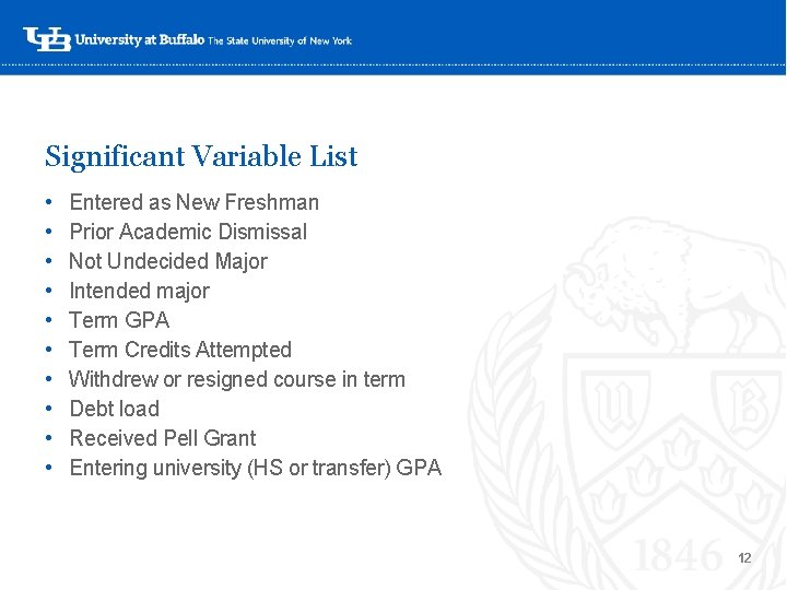
Significant Variable List • • • Entered as New Freshman Prior Academic Dismissal Not Undecided Major Intended major Term GPA Term Credits Attempted Withdrew or resigned course in term Debt load Received Pell Grant Entering university (HS or transfer) GPA ‘- 12

Results ‘- 13

Probability Scoring • After all of the models were complete and only significant variables remained in the equation, the probability scores were calculated for each model using an output function in SPSS and exported in an Excel file. ‘- • We will run the simulations on each of these models individually and compare the results to the expected returning student counts 14

Now that we know how we built our model… ‘- 15

Why should you use simulative analytics? • Allows for a range of possible outcomes • Useful when we realize that there are many potential outcomes, not a single one – like in student enrollments Major users of simulative analytics: ‘- 16

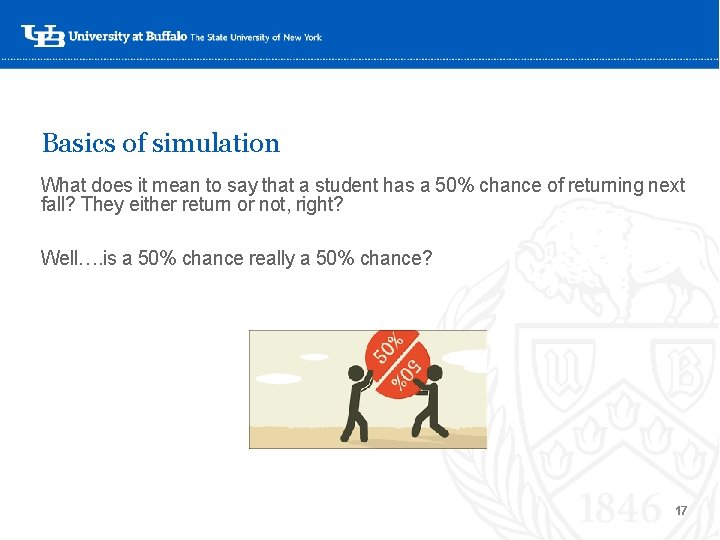
Basics of simulation What does it mean to say that a student has a 50% chance of returning next fall? They either return or not, right? Well…. is a 50% chance really a 50% chance? ‘- 17

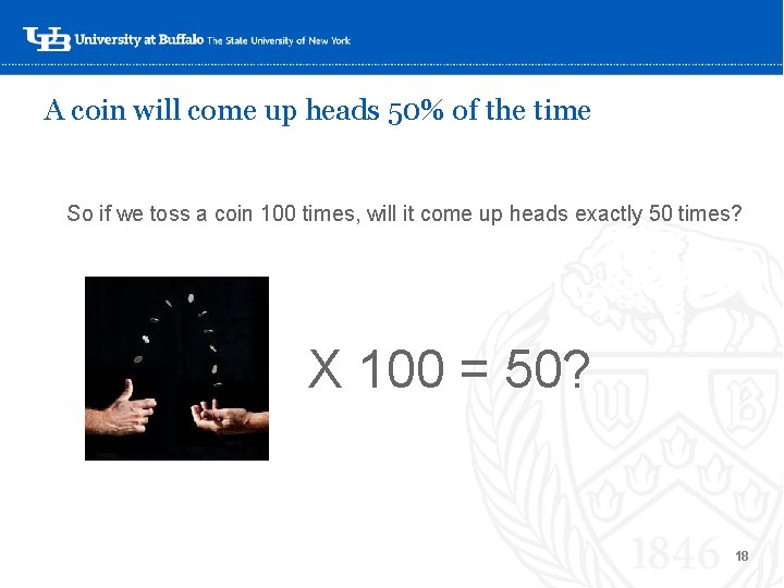
A coin will come up heads 50% of the time So if we toss a coin 100 times, will it come up heads exactly 50 times? ‘- X 100 = 50? 18

Using a confidence interval to identify a range • If we try throwing a coin 100 times, we’ll soon find out that heads don’t come up exactly 50 times in every attempt. • However, we can identify, within a certain range, ‘approximately how many times heads will come up in a certain percentage of attempts. This range is called the “confidence interval”. • Most confidence intervals are expressed within a percentage of 95%. • In other words, “ 95% of the time, heads will come up…” 19

Over the course of 100 throws, a coin will come up heads how many times? ‘- X 100 = 40 to 60 times 20

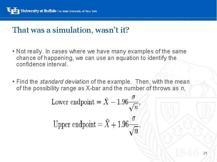
That was a simulation, wasn’t it? • Not really. In cases where we have many examples of the same chance of happening, we can use an equation to identify the confidence interval. ‘ • Find the standard deviation of the example. Then, with the mean of the possibility range as X-bar and the number of throws as n, 21

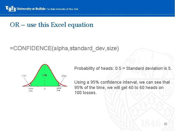
OR – use this Excel equation =CONFIDENCE(alpha, standard_dev, size) ‘Probability of heads: 0. 5 = Standard deviation is 5. Using a 95% confidence interval, we can see that 95% of the time, we will get 40 to 60 heads on 100 tosses. 22

What if… • The coin flip example is an event with only two possible outcomes. • We’ve got incidents with different probabilities—like students with different probabilities of returning, leading a lot‘-of possible outcomes – a range of potential enrollment totals. • The President/Provost/ Enrollment Planning want to know how likely it is that we’ll have 10, 000 continuing students. Or 12, 000…or 15, 000. • So – how can we do this? 23

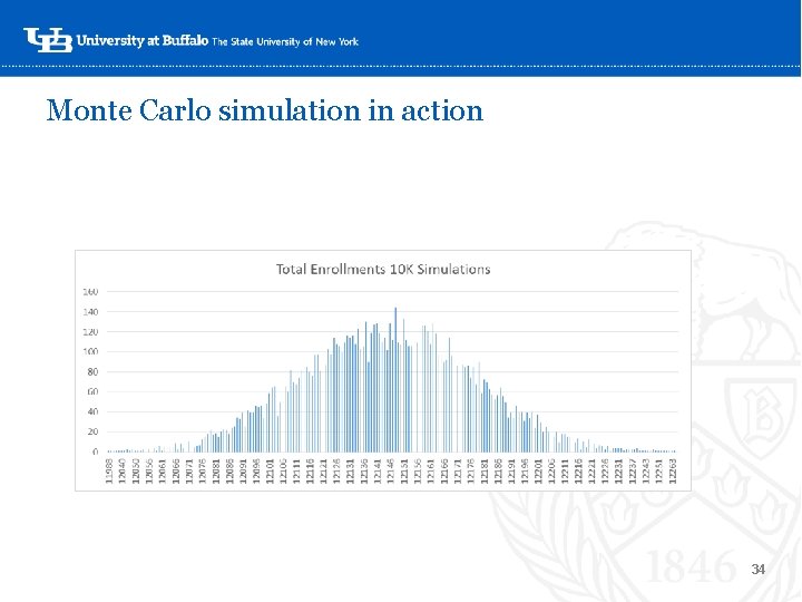
First, some vocabulary: • Simulation: Tossing a coin once. • Monte Carlo technique: Tossing 100 coins in the air at once. ‘- • Monte Carlo simulation: Simulate tossing 100 coins 10, 000 times. 24

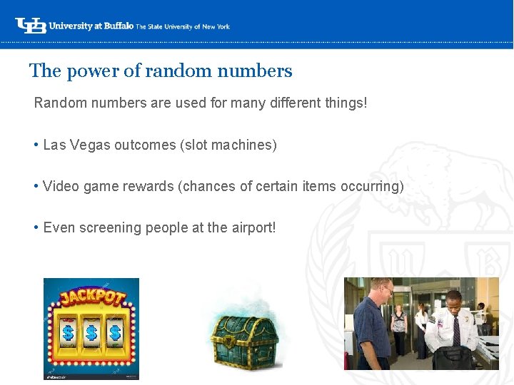
The power of random numbers Random numbers are used for many different things! • Las Vegas outcomes (slot machines) • Video game rewards (chances of certain items‘- occurring) • Even screening people at the airport! 25

Let Excel do the work! • The =RAND function will produce a random number, which is seeded to your computer’s internal clock ‘- 0 and 1 • This function returns a random fraction between • Our probability scores from the model are between 0 and 1… 26

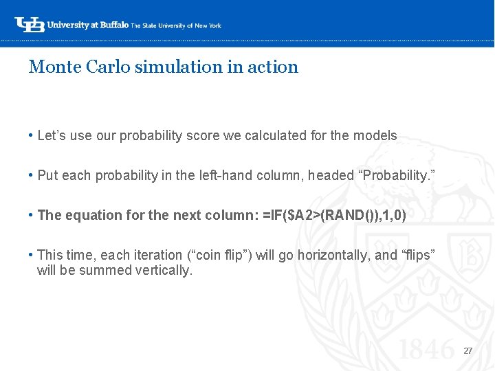
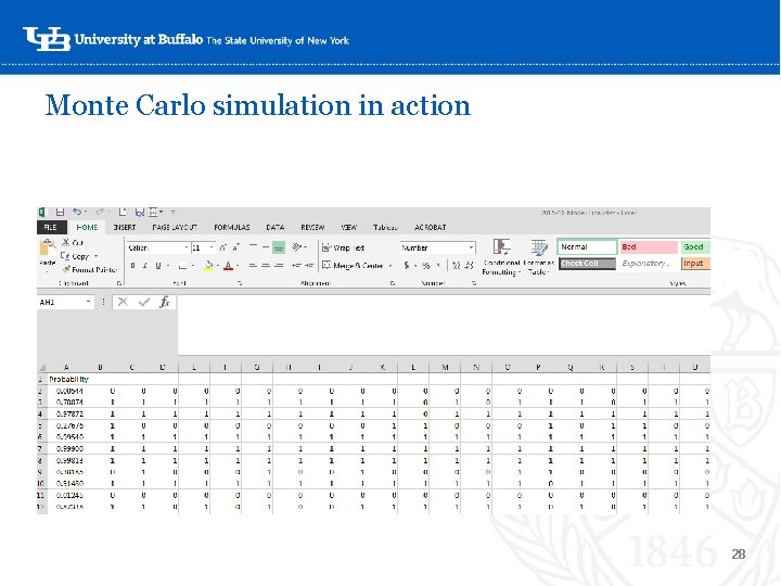
Monte Carlo simulation in action • Let’s use our probability score we calculated for the models • Put each probability in the left-hand column, headed “Probability. ” ‘- • The equation for the next column: =IF($A 2>(RAND()), 1, 0) • This time, each iteration (“coin flip”) will go horizontally, and “flips” will be summed vertically. 27

Monte Carlo simulation in action ‘- 28

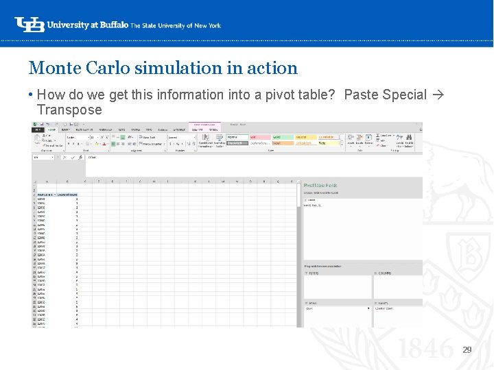
Monte Carlo simulation in action • How do we get this information into a pivot table? Paste Special Transpose ‘- 29

Monte Carlo simulation in action Want more simulations? • You don’t need to redo the formulas, just Recalculate. Excel will re ‘-seed the formulas and re-randomize the results. • Using the pivot table, we can figure out what our chances are of reaching a goal. You can even change the pivot table to percentage of total “flips” to make it easier. 30

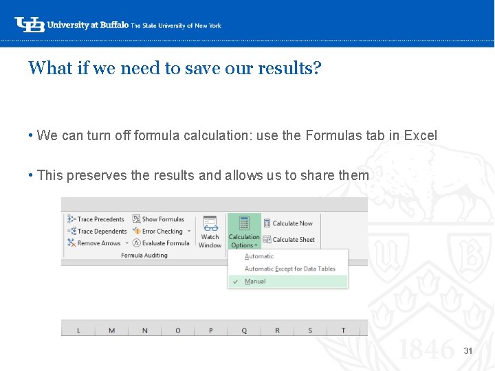
What if we need to save our results? • We can turn off formula calculation: use the Formulas tab in Excel • This preserves the results and allows us to share them ‘- 31

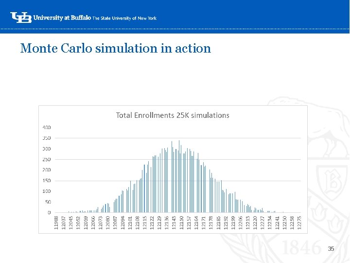
And now, a brief aside about anomalies • It is human nature to look for anomalies or things that “stand out” in the data. For example – the one simulation where very few or almost all of the students returned. ‘- • Don’t do this in simulative analytics. A handful of random numbers that appear to have meaning probably won’t when that randomization is repeated thousands of times. • This is why we recommend running the simulation at least 10, 000 times, and preferably for 25, 000. Anomalies will be “smoothed” out in the masses of results. 32

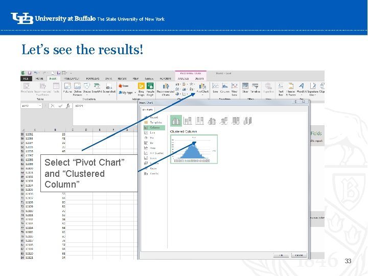
Let’s see the results! ‘Select “Pivot Chart” and “Clustered Column” 33

Monte Carlo simulation in action ‘- 34

Monte Carlo simulation in action ‘- 35

Use and Implications • Adjusting the model: what we’ve found to work, and what might not • Impact of policy changes (Finish in 4, Excelsior Scholarship) • Students now have more incentives to stay enrolled at a certain level ‘ • Excelsior program may mean debt indicators take on a different importance • Ways to expand: graduate and professional enrollments? • Can we come up with a model that works across programs? 36

Questions? Feedback? ‘- Michael Randall mrandall@buffalo. edu Rachel Link rlink 2@buffalo. edu 37