ENPH 259 201213 term 1 Homework problem set

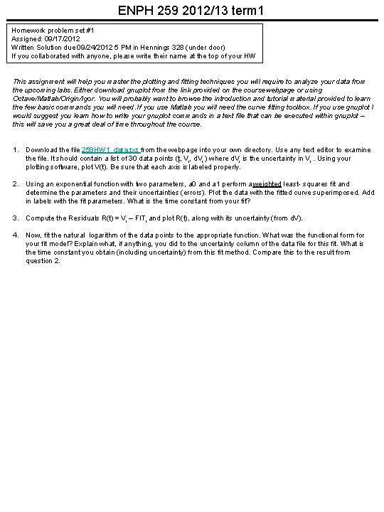
ENPH 259 2012/13 term 1 Homework problem set #1 Assigned: 09/17/2012 Written Solution due 09/24/2012 5 PM in Hennings 328 (under door) If you collaborated with anyone, please write their name at the top of your HW This assignment will help you master the plotting and fitting techniques you will require to analyze your data from the upcoming labs. Either download gnuplot from the link provided on the course webpage or using Octave/Matlab/Origin/Igor. You will probably want to browse the introduction and tutorial material provided to learn the few basic commands you will need. If you use Matlab you will need the curve fitting toolbox. If you use gnuplot I would suggest you learn how to write your gnuplot commands in a text file that can be executed within gnuplot – this will save you a great deal of time throughout the course. 1. Download the file 259 HW 1_data. txt from the webpage into your own directory. Use any text editor to examine the file. It should contain a list of 30 data points (ti, Vi, d. Vi ) where d. Vi is the uncertainty in Vi. Using your plotting software, plot V(t). Be sure that each axis is labeled properly. 2. Using an exponential function with two parameters, a 0 and a 1 perform a weighted least- squares fit and determine the parameters and their uncertainties (errors). Plot the data with the fitted curve superimposed. Add in labels with the fit parameters. What is the time constant from your fit? 3. Compute the Residuals R(t) = Vi – FITi and plot R(t), along with its uncertainty (from d. V). 4. Now, fit the natural logarithm of the data points to the appropriate function. What was the functional form for your fit model? Explain what, if anything, you did to the uncertainty column of the data file for this fit. What is the time constant you obtain (including uncertainty) from this fit method. Compare this to the result from question 2.