ENGMAE 200 A Engineering Analysis I Matrix Eigenvalue

ENGMAE 200 A: Engineering Analysis I Matrix Eigenvalue Problems Instructor: Dr. Ramin Bostanabad

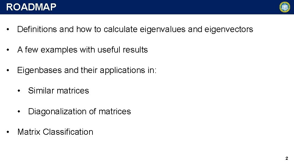
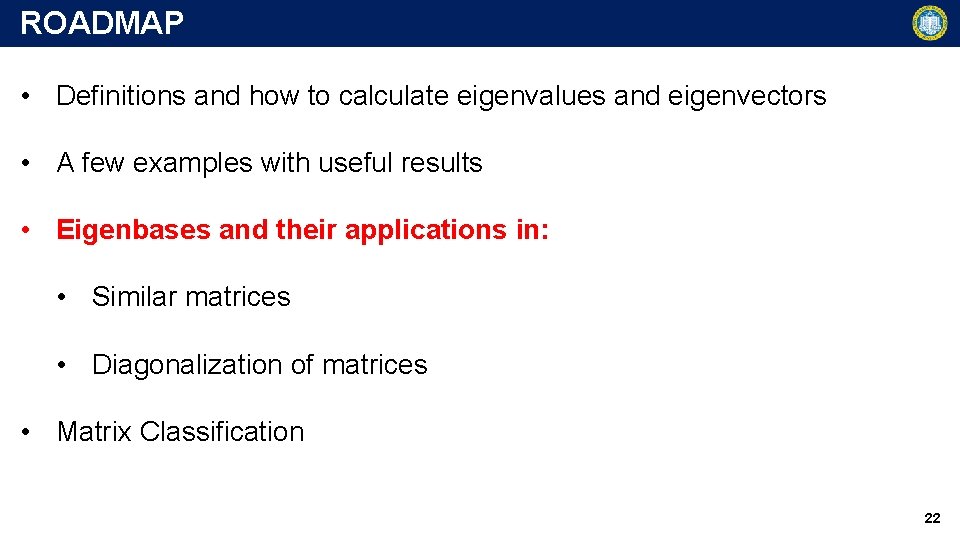
ROADMAP • Definitions and how to calculate eigenvalues and eigenvectors • A few examples with useful results • Eigenbases and their applications in: • Similar matrices • Diagonalization of matrices • Matrix Classification 2

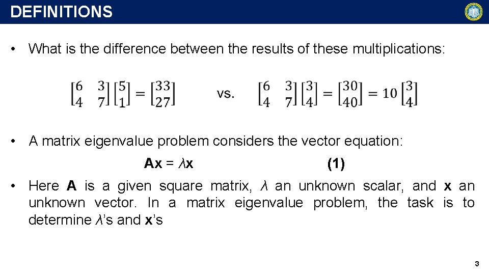
DEFINITIONS • What is the difference between the results of these multiplications: • A matrix eigenvalue problem considers the vector equation: Ax = λx (1) • Here A is a given square matrix, λ an unknown scalar, and x an unknown vector. In a matrix eigenvalue problem, the task is to determine λ’s and x’s 3

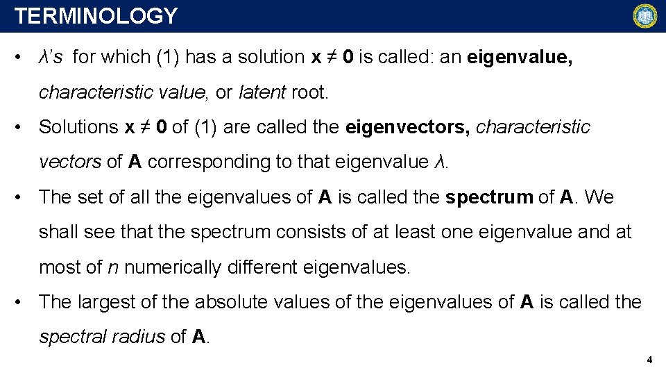
TERMINOLOGY • λ’s for which (1) has a solution x ≠ 0 is called: an eigenvalue, characteristic value, or latent root. • Solutions x ≠ 0 of (1) are called the eigenvectors, characteristic vectors of A corresponding to that eigenvalue λ. • The set of all the eigenvalues of A is called the spectrum of A. We shall see that the spectrum consists of at least one eigenvalue and at most of n numerically different eigenvalues. • The largest of the absolute values of the eigenvalues of A is called the spectral radius of A. 4

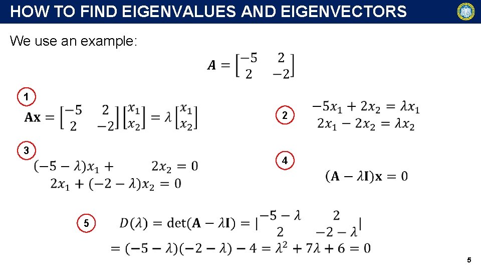
HOW TO FIND EIGENVALUES AND EIGENVECTORS We use an example: 1 2 3 4 5 5

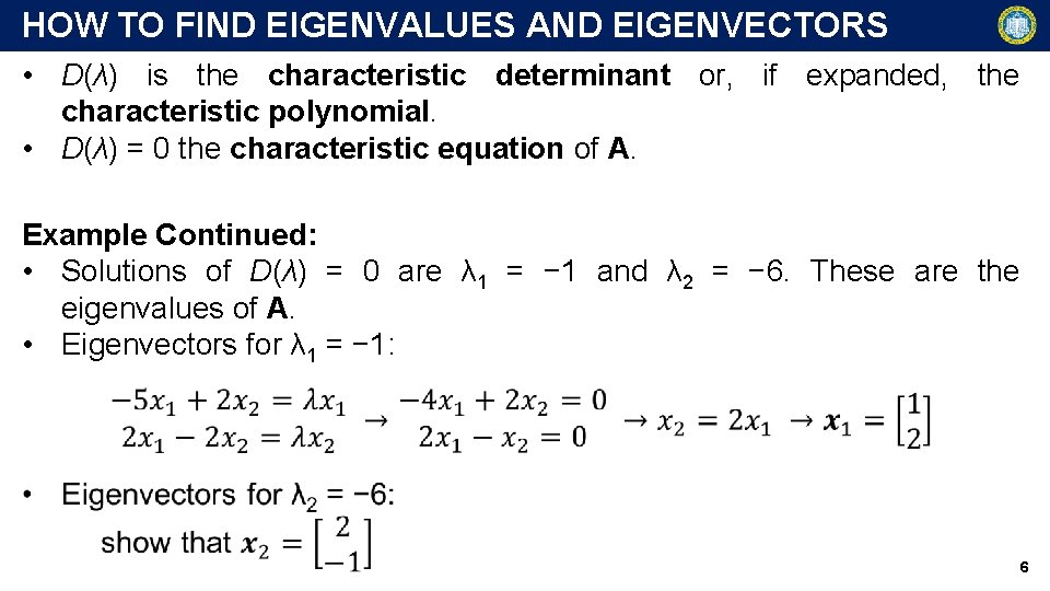
HOW TO FIND EIGENVALUES AND EIGENVECTORS • D(λ) is the characteristic determinant or, if expanded, the characteristic polynomial. • D(λ) = 0 the characteristic equation of A. Example Continued: • Solutions of D(λ) = 0 are λ 1 = − 1 and λ 2 = − 6. These are the eigenvalues of A. • Eigenvectors for λ 1 = − 1: 6

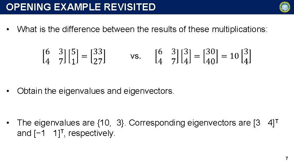
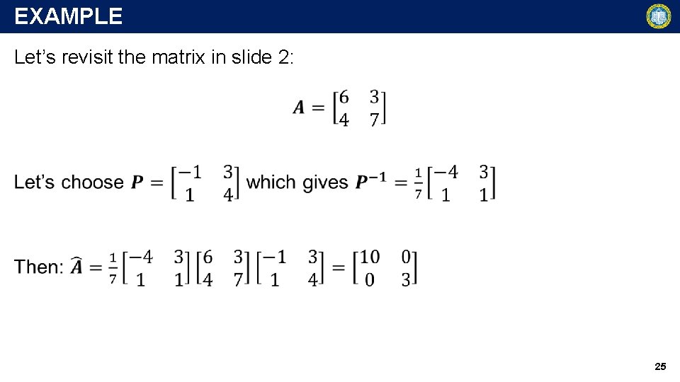
OPENING EXAMPLE REVISITED • What is the difference between the results of these multiplications: • Obtain the eigenvalues and eigenvectors. • The eigenvalues are {10, 3}. Corresponding eigenvectors are [3 4]T and [− 1 1]T, respectively. 7

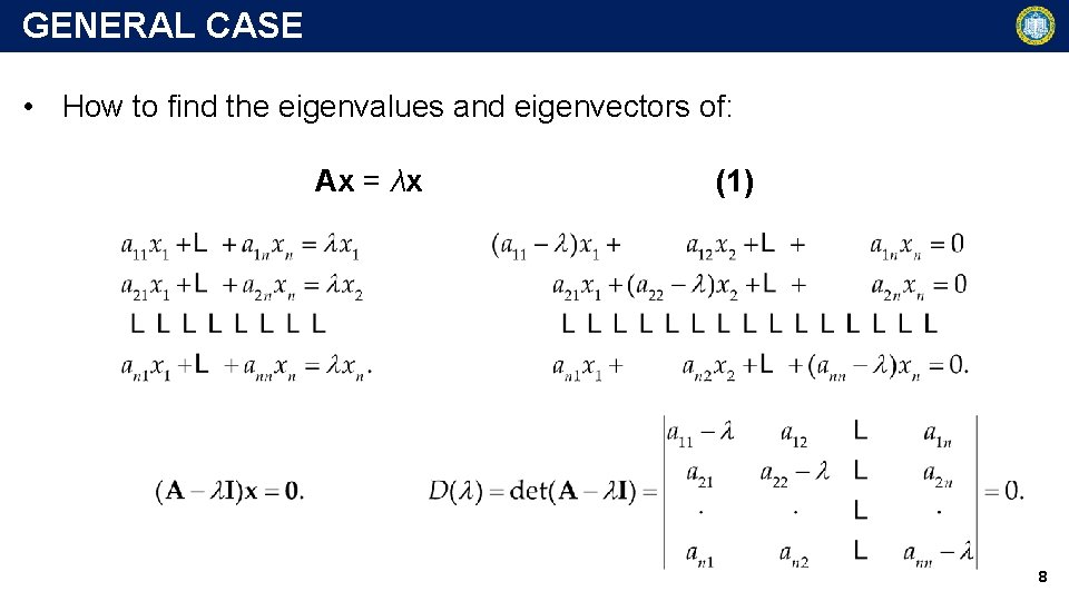
GENERAL CASE • How to find the eigenvalues and eigenvectors of: Ax = λx (1) 8

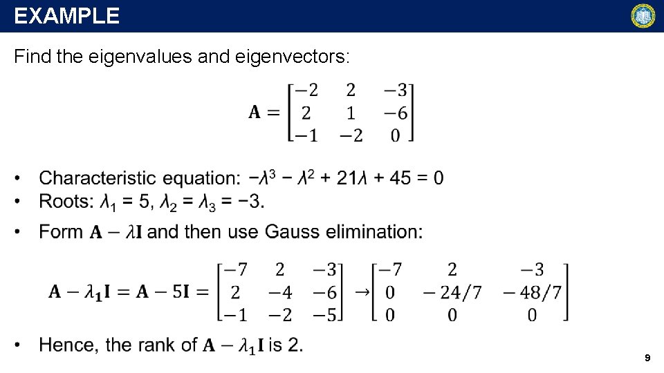
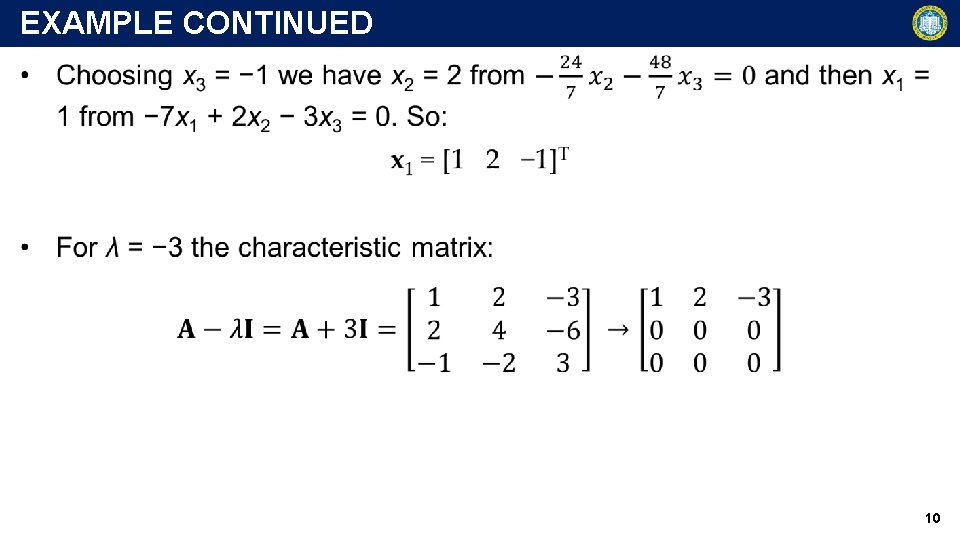
EXAMPLE Find the eigenvalues and eigenvectors: 9

EXAMPLE CONTINUED 10

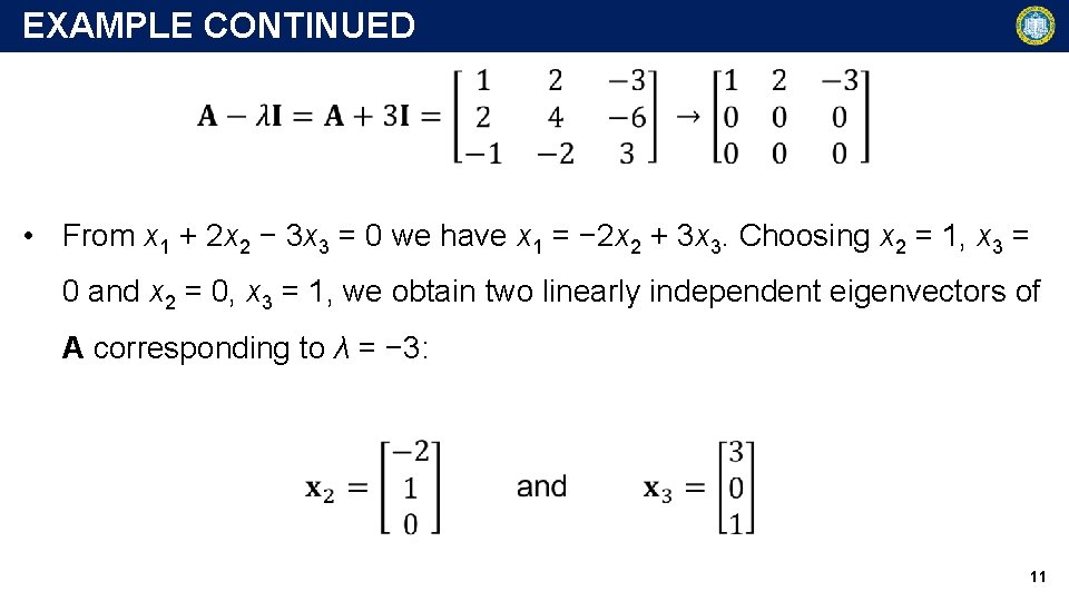
EXAMPLE CONTINUED • From x 1 + 2 x 2 − 3 x 3 = 0 we have x 1 = − 2 x 2 + 3 x 3. Choosing x 2 = 1, x 3 = 0 and x 2 = 0, x 3 = 1, we obtain two linearly independent eigenvectors of A corresponding to λ = − 3: 11

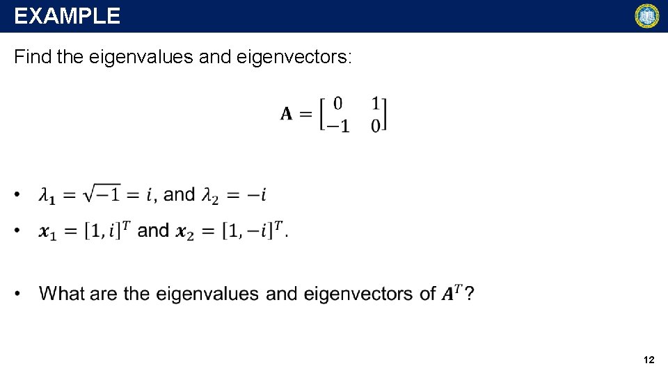
EXAMPLE Find the eigenvalues and eigenvectors: 12

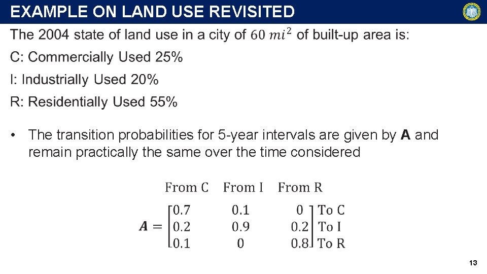
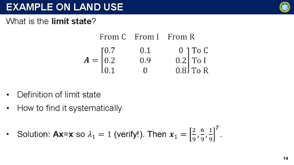
EXAMPLE ON LAND USE REVISITED • The transition probabilities for 5 -year intervals are given by A and remain practically the same over the time considered 13

EXAMPLE ON LAND USE What is the limit state? • Definition of limit state • How to find it systematically 14

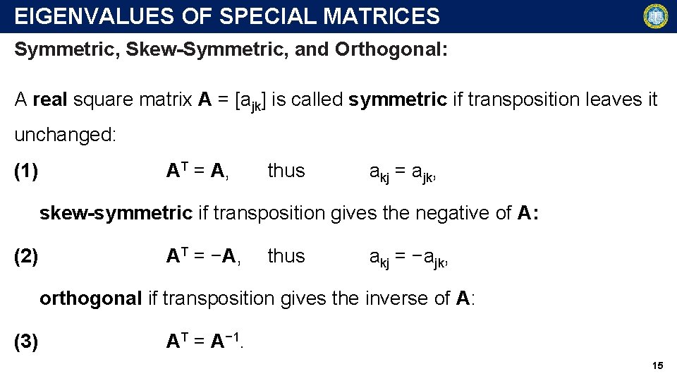
EIGENVALUES OF SPECIAL MATRICES Symmetric, Skew-Symmetric, and Orthogonal: A real square matrix A = [ajk] is called symmetric if transposition leaves it unchanged: (1) AT = A, thus akj = ajk, skew-symmetric if transposition gives the negative of A: (2) AT = −A, thus akj = −ajk, orthogonal if transposition gives the inverse of A: (3) AT = A− 1. 15

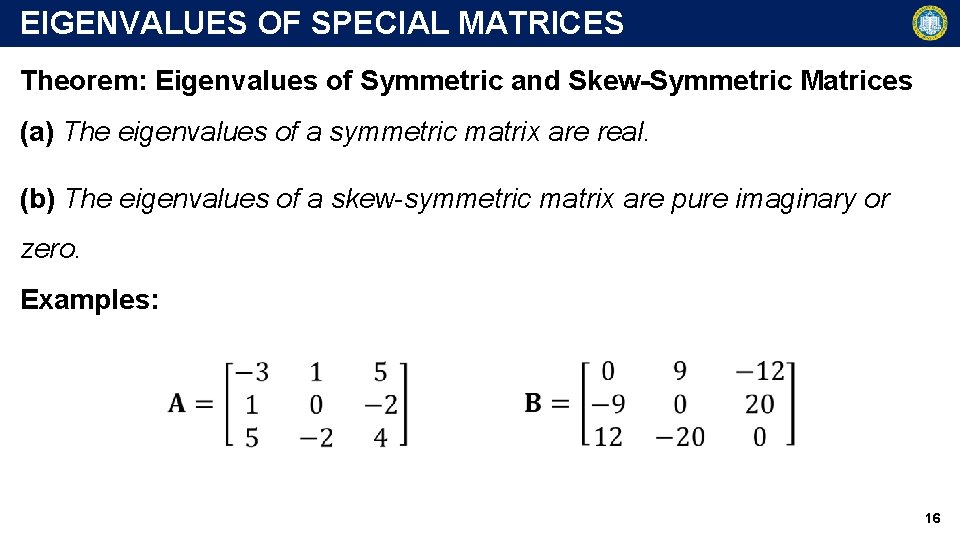
EIGENVALUES OF SPECIAL MATRICES Theorem: Eigenvalues of Symmetric and Skew-Symmetric Matrices (a) The eigenvalues of a symmetric matrix are real. (b) The eigenvalues of a skew-symmetric matrix are pure imaginary or zero. Examples: 16

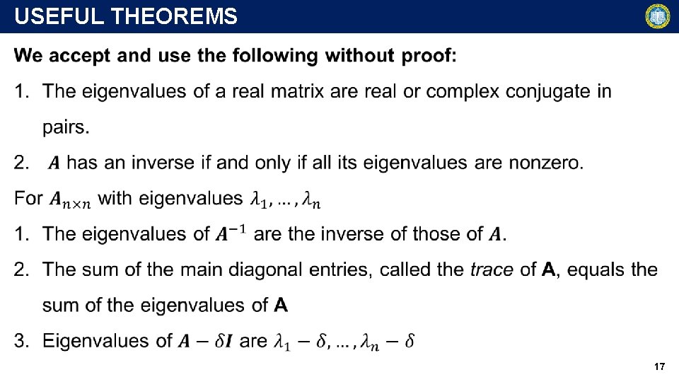
USEFUL THEOREMS 17

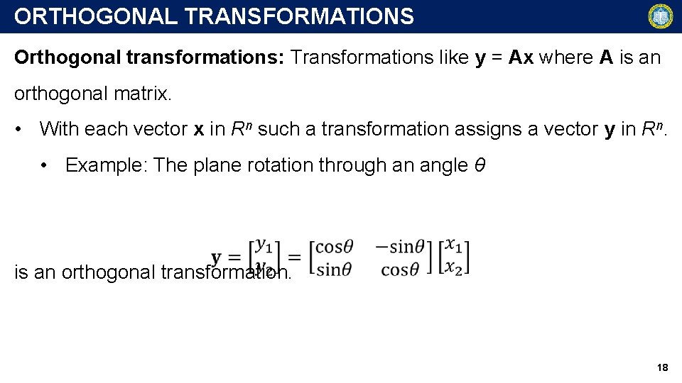
ORTHOGONAL TRANSFORMATIONS Orthogonal transformations: Transformations like y = Ax where A is an orthogonal matrix. • With each vector x in Rn such a transformation assigns a vector y in Rn. • Example: The plane rotation through an angle θ is an orthogonal transformation. 18

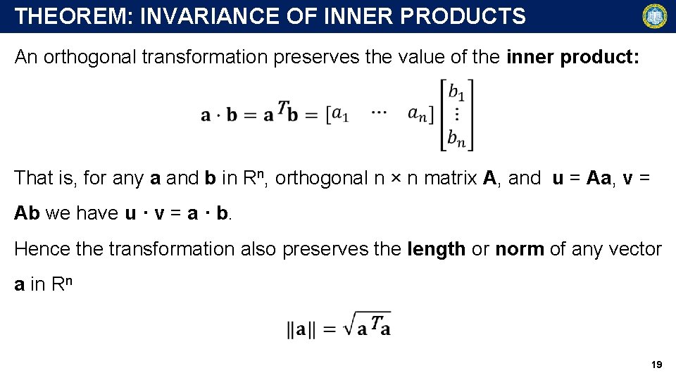
THEOREM: INVARIANCE OF INNER PRODUCTS An orthogonal transformation preserves the value of the inner product: That is, for any a and b in Rn, orthogonal n × n matrix A, and u = Aa, v = Ab we have u · v = a · b. Hence the transformation also preserves the length or norm of any vector a in Rn 19

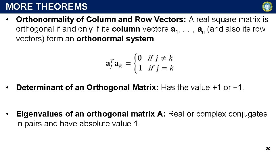
MORE THEOREMS • Orthonormality of Column and Row Vectors: A real square matrix is orthogonal if and only if its column vectors a 1, … , an (and also its row vectors) form an orthonormal system: • Determinant of an Orthogonal Matrix: Has the value +1 or − 1. • Eigenvalues of an orthogonal matrix A: Real or complex conjugates in pairs and have absolute value 1. 20

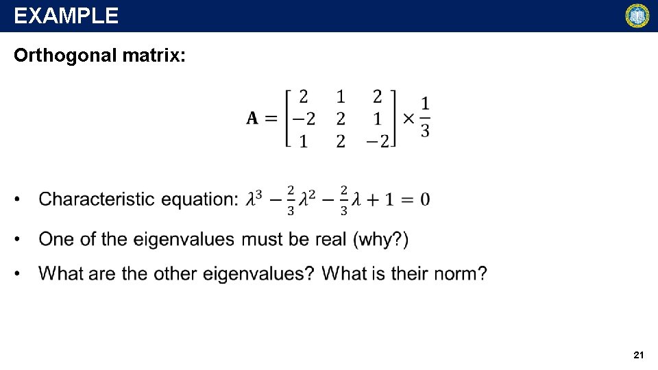
EXAMPLE Orthogonal matrix: 21

ROADMAP • Definitions and how to calculate eigenvalues and eigenvectors • A few examples with useful results • Eigenbases and their applications in: • Similar matrices • Diagonalization of matrices • Matrix Classification 22

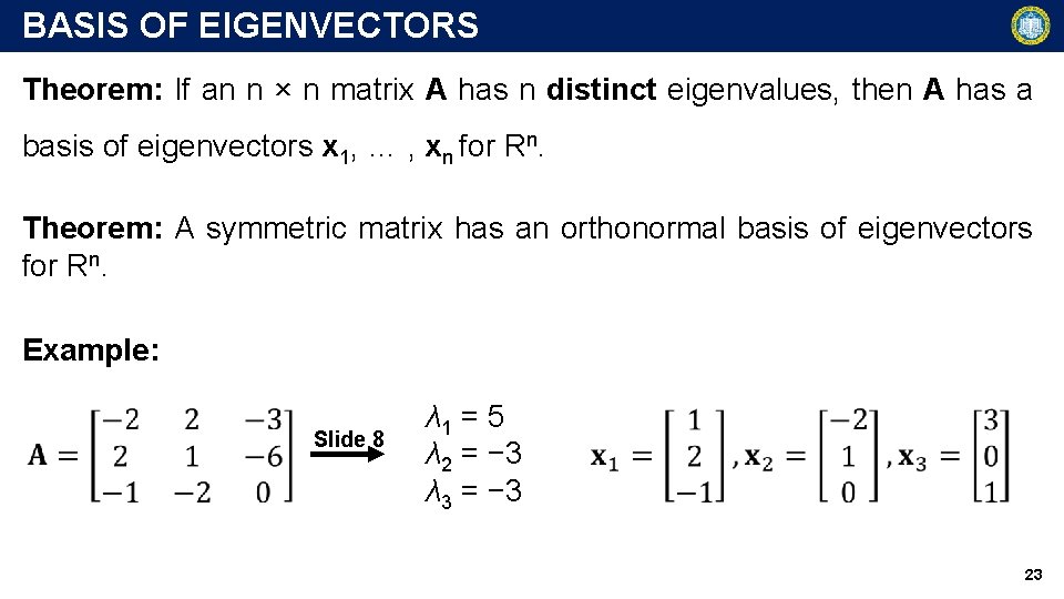
BASIS OF EIGENVECTORS Theorem: If an n × n matrix A has n distinct eigenvalues, then A has a basis of eigenvectors x 1, … , xn for Rn. Theorem: A symmetric matrix has an orthonormal basis of eigenvectors for Rn. Example: Slide 8 λ 1 = 5 λ 2 = − 3 λ 3 = − 3 23

SIMILARITY OF MATRICES Definition: An n × n matrix is called similar to an n × n matrix A if = P− 1 AP for some (nonsingular!) n × n matrix P. This transformation, which gives from A, is called a similarity transformation. Theorem: If is similar to A, then has the same eigenvalues as A. Furthermore, if x is an eigenvector of A, then y = P− 1 x is an eigenvector of corresponding to the same eigenvalue. 24

EXAMPLE Let’s revisit the matrix in slide 2: 25

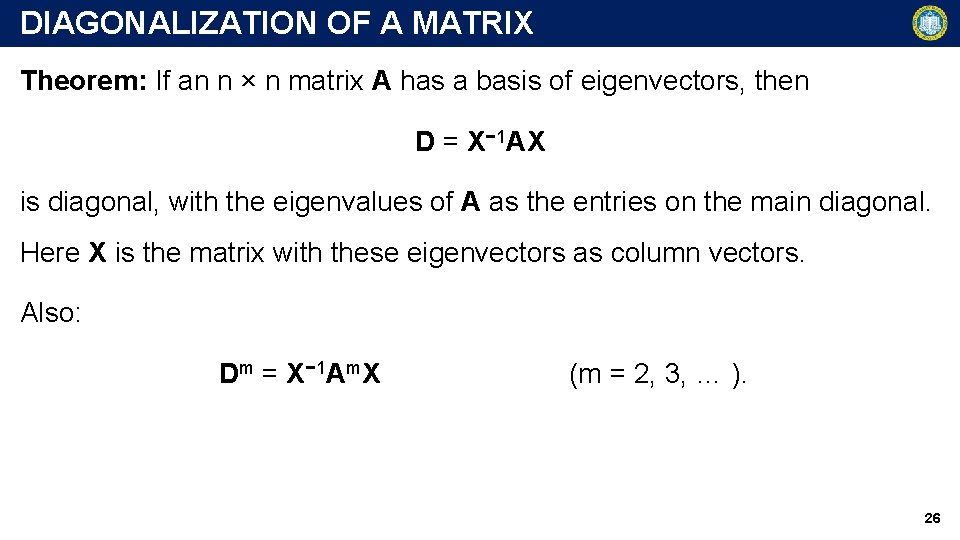
DIAGONALIZATION OF A MATRIX Theorem: If an n × n matrix A has a basis of eigenvectors, then D = X− 1 AX is diagonal, with the eigenvalues of A as the entries on the main diagonal. Here X is the matrix with these eigenvectors as column vectors. Also: Dm = X− 1 Am. X (m = 2, 3, … ). 26

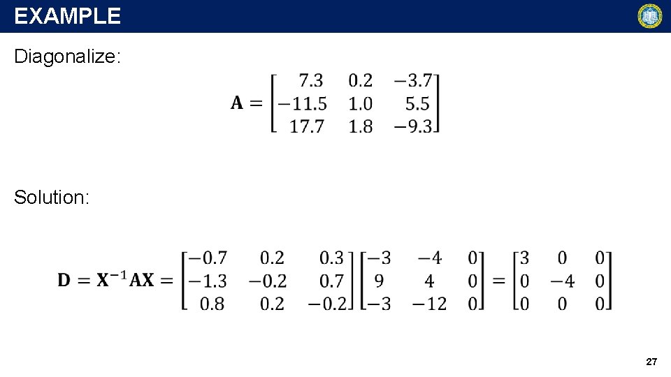
EXAMPLE Diagonalize: Solution: 27

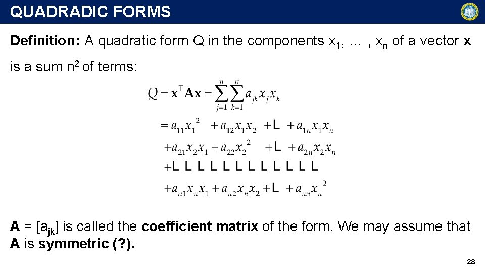
QUADRADIC FORMS Definition: A quadratic form Q in the components x 1, … , xn of a vector x is a sum n 2 of terms: A = [ajk] is called the coefficient matrix of the form. We may assume that A is symmetric (? ). 28

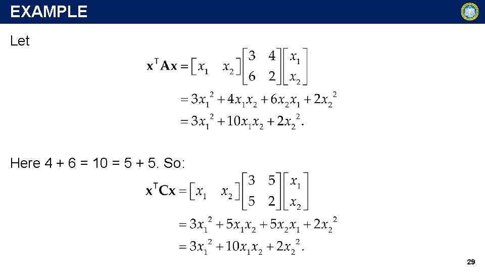
EXAMPLE Let Here 4 + 6 = 10 = 5 + 5. So: 29

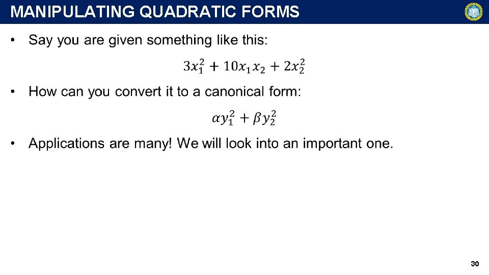
MANIPULATING QUADRATIC FORMS 30

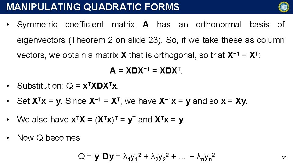
MANIPULATING QUADRATIC FORMS • Symmetric coefficient matrix A has an orthonormal basis of eigenvectors (Theorem 2 on slide 23). So, if we take these as column vectors, we obtain a matrix X that is orthogonal, so that X− 1 = XT: A = XDX− 1 = XDXT. • Substitution: Q = x. TXDXTx. • Set XTx = y. Since X− 1 = XT, we have X− 1 x = y and so x = Xy. • We also have x. TX = (XTx)T = y. T and XTx = y. • Now Q becomes Q = y. TDy = λ 1 y 12 + λ 2 y 22 + … + λnyn 2 31

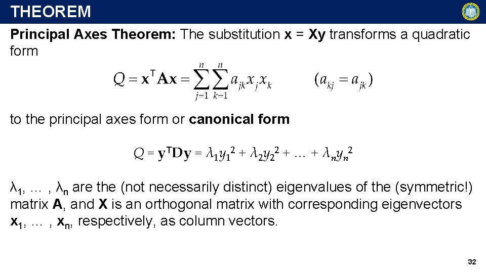
THEOREM Principal Axes Theorem: The substitution x = Xy transforms a quadratic form to the principal axes form or canonical form Q = y. TDy = λ 1 y 12 + λ 2 y 22 + … + λnyn 2 λ 1, … , λn are the (not necessarily distinct) eigenvalues of the (symmetric!) matrix A, and X is an orthogonal matrix with corresponding eigenvectors x 1, … , xn, respectively, as column vectors. 32

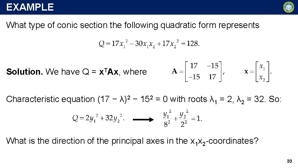
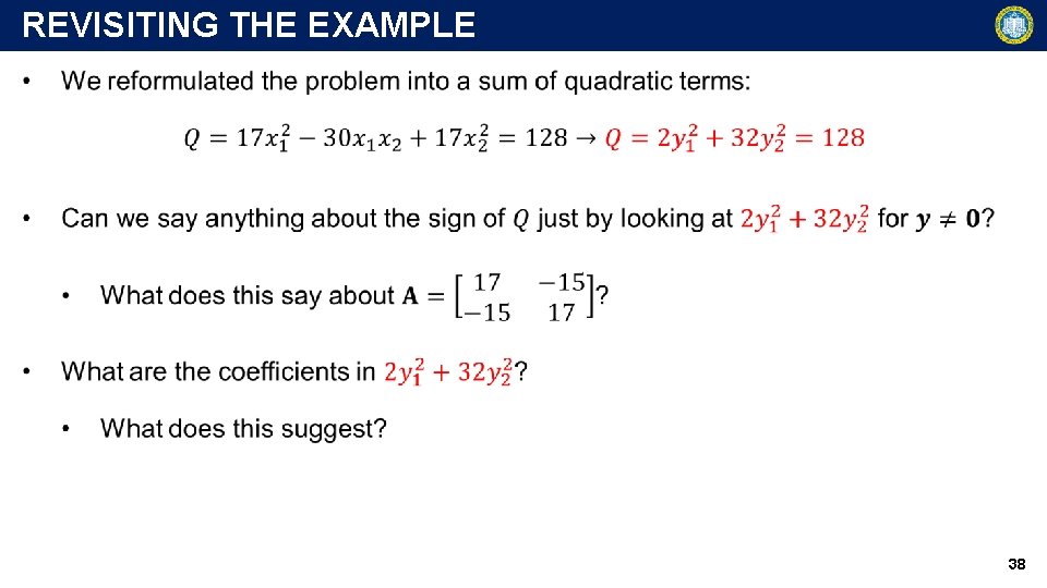
EXAMPLE What type of conic section the following quadratic form represents Solution. We have Q = x. TAx, where Characteristic equation (17 − λ)2 − 152 = 0 with roots λ 1 = 2, λ 2 = 32. So: What is the direction of the principal axes in the x 1 x 2 -coordinates? 33

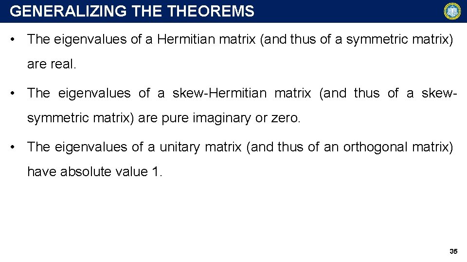
COMPLEX MATRICES A square matrix A = [akj] is called Hermitian if ĀT = A, that is, ākj = ajk skew-Hermitian if ĀT = −A, that is, ākj = −ajk unitary if ĀT = A− 1 • These are generalization of symmetric, skew-symmetric, and orthogonal matrices in complex spaces. • For example (Theorem on invariance of Inner Product): The unitary transformation y = Ax with a unitary matrix A, preserves the value of the inner product and norm. 34

GENERALIZING THEOREMS • The eigenvalues of a Hermitian matrix (and thus of a symmetric matrix) are real. • The eigenvalues of a skew-Hermitian matrix (and thus of a skewsymmetric matrix) are pure imaginary or zero. • The eigenvalues of a unitary matrix (and thus of an orthogonal matrix) have absolute value 1. 35

ROADMAP • Definitions and how to calculate eigenvalues and eigenvectors • A few examples with useful results • Eigenbases and their applications in: • Similar matrices • Diagonalization of matrices • Matrix Classification 36

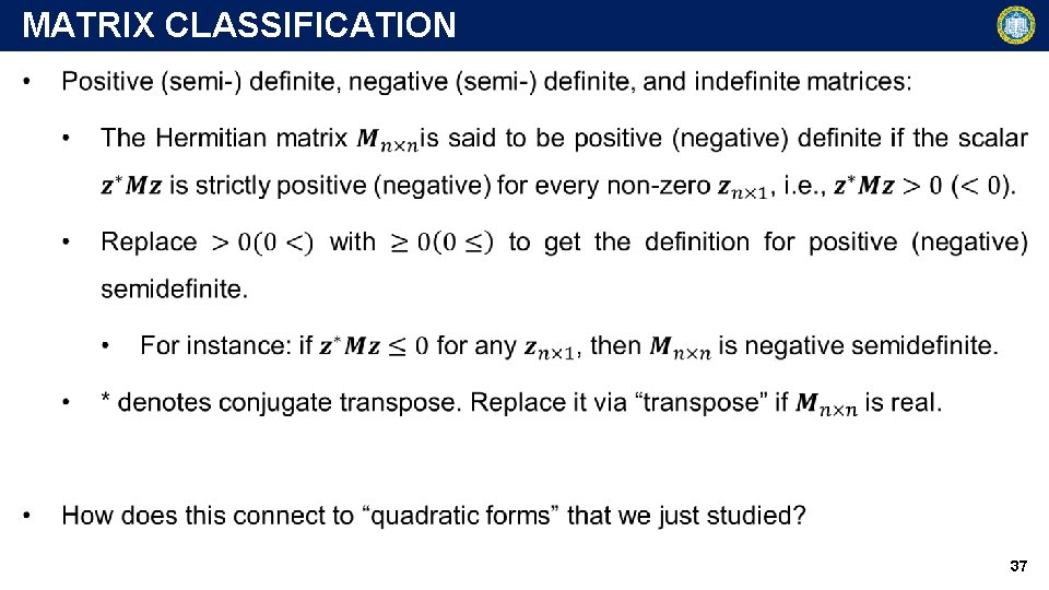
MATRIX CLASSIFICATION 37

REVISITING THE EXAMPLE 38

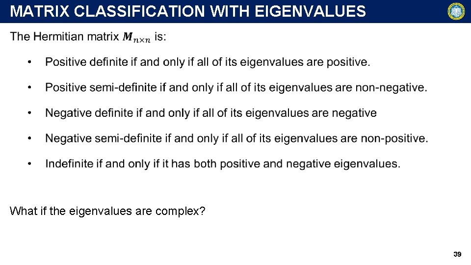
MATRIX CLASSIFICATION WITH EIGENVALUES What if the eigenvalues are complex? 39

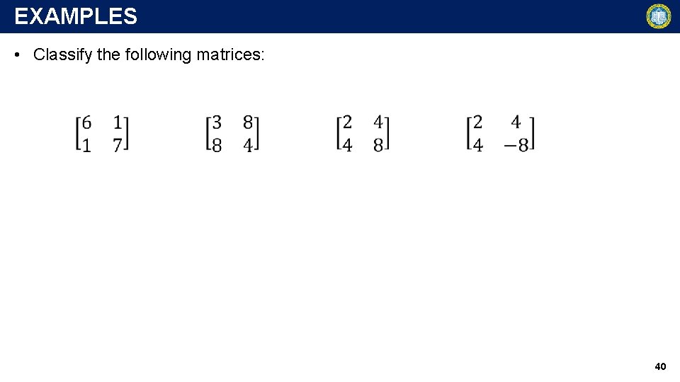
EXAMPLES • Classify the following matrices: 40

EXTRA 41

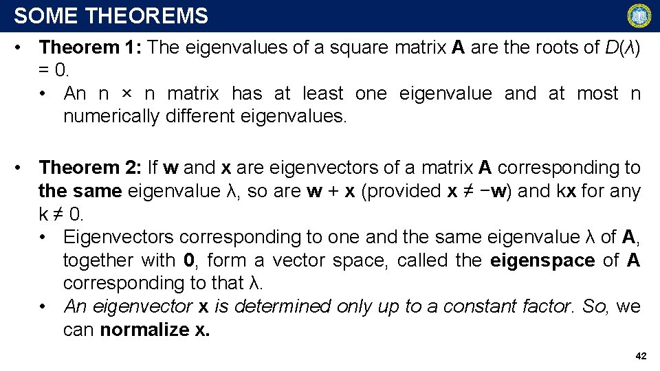
SOME THEOREMS • Theorem 1: The eigenvalues of a square matrix A are the roots of D(λ) = 0. • An n × n matrix has at least one eigenvalue and at most n numerically different eigenvalues. • Theorem 2: If w and x are eigenvectors of a matrix A corresponding to the same eigenvalue λ, so are w + x (provided x ≠ −w) and kx for any k ≠ 0. • Eigenvectors corresponding to one and the same eigenvalue λ of A, together with 0, form a vector space, called the eigenspace of A corresponding to that λ. • An eigenvector x is determined only up to a constant factor. So, we can normalize x. 42