
ENGINEERING MATHEMATICS II MA2001 Dr Umber Sheikh Course
ENGINEERING MATHEMATICS II MA-2001 Dr. Umber Sheikh
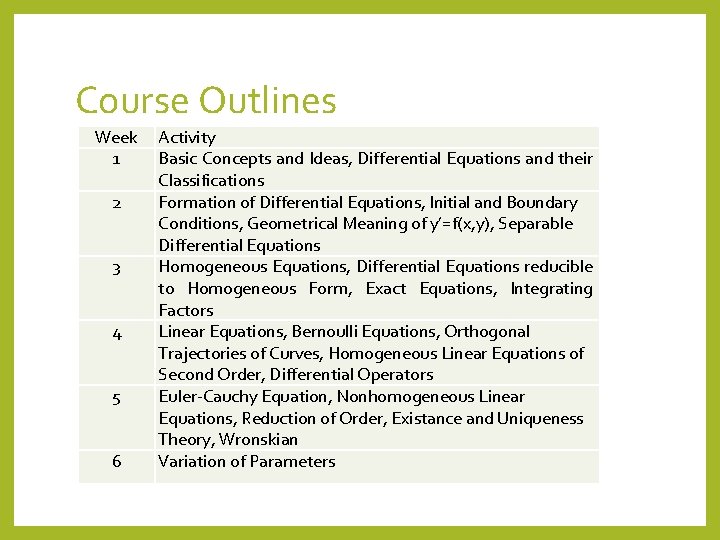
Course Outlines Week 1 2 3 4 5 6 Activity Basic Concepts and Ideas, Differential Equations and their Classifications Formation of Differential Equations, Initial and Boundary Conditions, Geometrical Meaning of y’=f(x, y), Separable Differential Equations Homogeneous Equations, Differential Equations reducible to Homogeneous Form, Exact Equations, Integrating Factors Linear Equations, Bernoulli Equations, Orthogonal Trajectories of Curves, Homogeneous Linear Equations of Second Order, Differential Operators Euler-Cauchy Equation, Nonhomogeneous Linear Equations, Reduction of Order, Existance and Uniqueness Theory, Wronskian Variation of Parameters
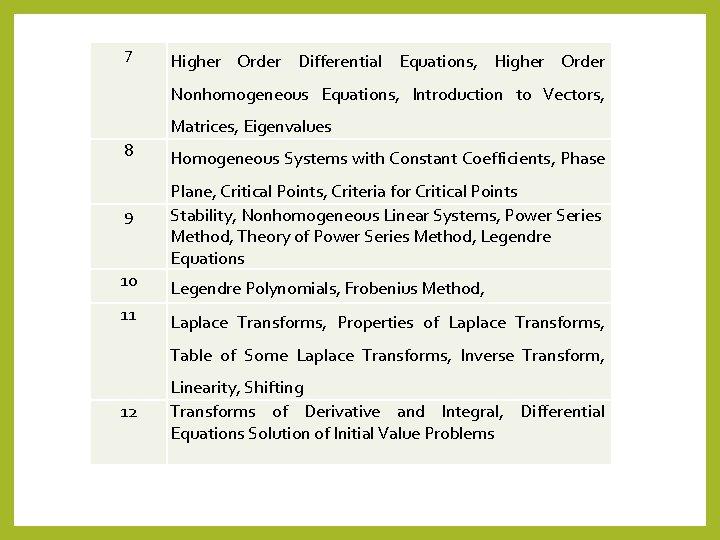
7 Higher Order Differential Equations, Higher Order Nonhomogeneous Equations, Introduction to Vectors, Matrices, Eigenvalues 8 9 10 11 Homogeneous Systems with Constant Coefficients, Phase Plane, Critical Points, Criteria for Critical Points Stability, Nonhomogeneous Linear Systems, Power Series Method, Theory of Power Series Method, Legendre Equations Legendre Polynomials, Frobenius Method, Laplace Transforms, Properties of Laplace Transforms, Table of Some Laplace Transforms, Inverse Transform, 12 Linearity, Shifting Transforms of Derivative and Integral, Differential Equations Solution of Initial Value Problems
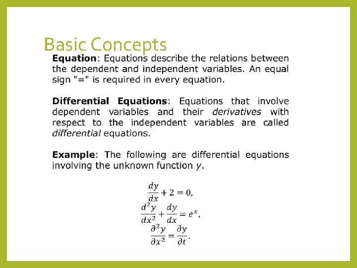
Basic Concepts
Some Other Examples: Newton’s Second Law of Motion Maxwell Equations Kirchhoff’s Laws Heat Equation Wave Equation Ordinary Differential Equation: Differential equations that involve only one independent variable are called ordinary differential equations. Partial Differential Equation: Differential equations that involve two or more independent variables are called partial differential equations. Examples: Equations 1 and 2 are examples of ordinary differential equations, since the unknown function y depends solely on the variable x. Equation 3 is a partial differential equation, since y depends on both the independent variables t and x.
Order: The order of a differential equation is the highest derivative that appears in the differential equation. Degree: The degree of a differential equation is the power of the highest derivative term. Linear Equations: A differential equation is called linear if there are no multiplications among dependent variables and their derivatives. In other words, all coefficients are functions of independent variables. Non-linear: Differential equations that do not satisfy the definition of linear are non-linear.
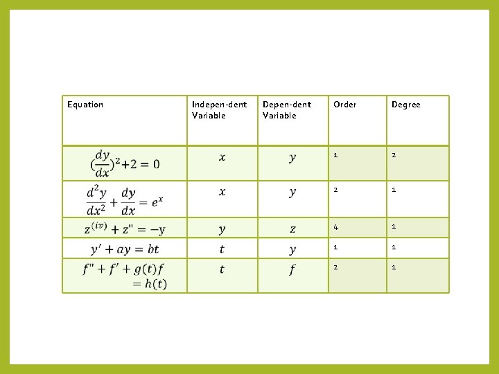
Equation Indepen-dent Variable Depen-dent Variable Order Degree 1 2 2 1 4 1 1 1 2 1
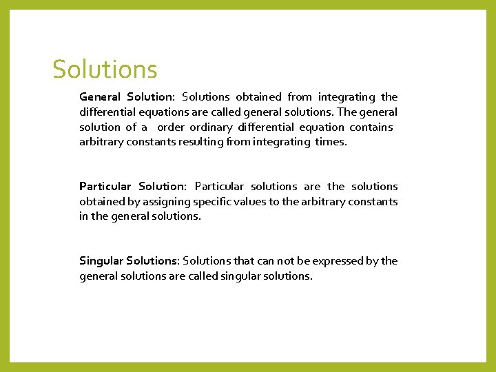
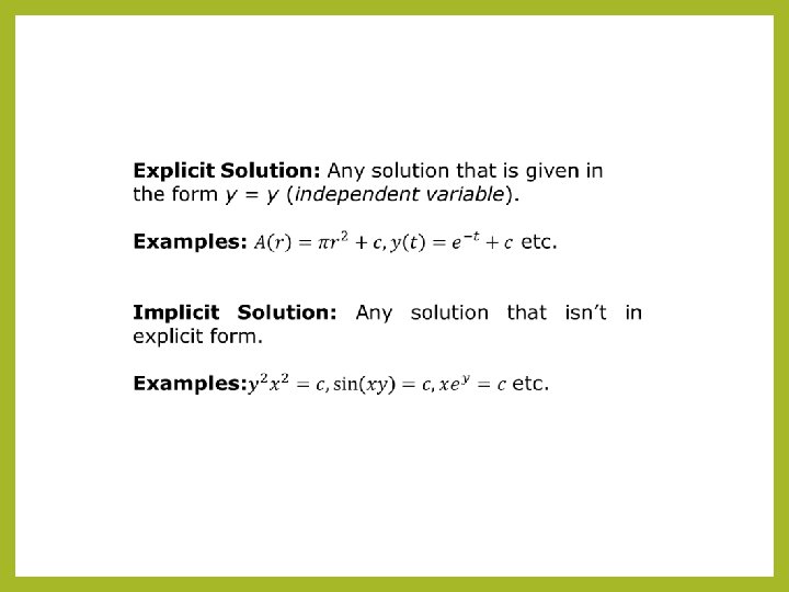
Solutions General Solution: Solutions obtained from integrating the differential equations are called general solutions. The general solution of a order ordinary differential equation contains arbitrary constants resulting from integrating times. Particular Solution: Particular solutions are the solutions obtained by assigning specific values to the arbitrary constants in the general solutions. Singular Solutions: Solutions that can not be expressed by the general solutions are called singular solutions.
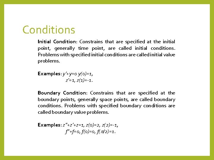
Conditions Initial Condition: Constrains that are specified at the initial point, generally time point, are called initial conditions. Problems with specified initial conditions are called initial value problems. Examples: y’+y=0 y(0)=1, z’=1, z(1)=-1. Boundary Condition: Constrains that are specified at the boundary points, generally space points, are called boundary conditions. Problems with specified boundary conditions are called boundary value problems. Examples: z”+z’+z=1, z(0)=2, z(2)=-1, f”+f=0, f(0)=0, f( /2)=1.

Worksheet 1 Equation Independent Variable Dependent Variable Order Degree Homo-genity
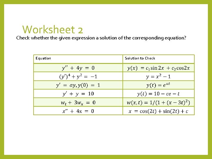
Worksheet 2 Check whether the given expression a solution of the corresponding equation? Equation Solution to Check
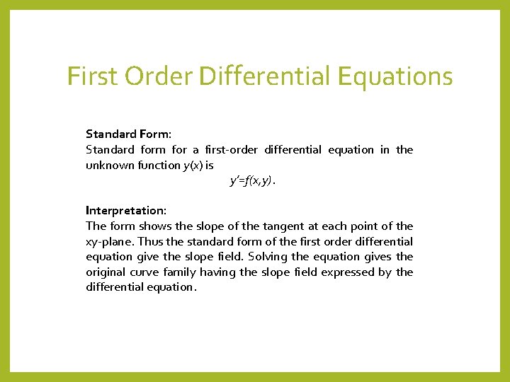
First Order Differential Equations Standard Form: Standard form for a first-order differential equation in the unknown function y(x) is y’=f(x, y). Interpretation: The form shows the slope of the tangent at each point of the xy-plane. Thus the standard form of the first order differential equation give the slope field. Solving the equation gives the original curve family having the slope field expressed by the differential equation.
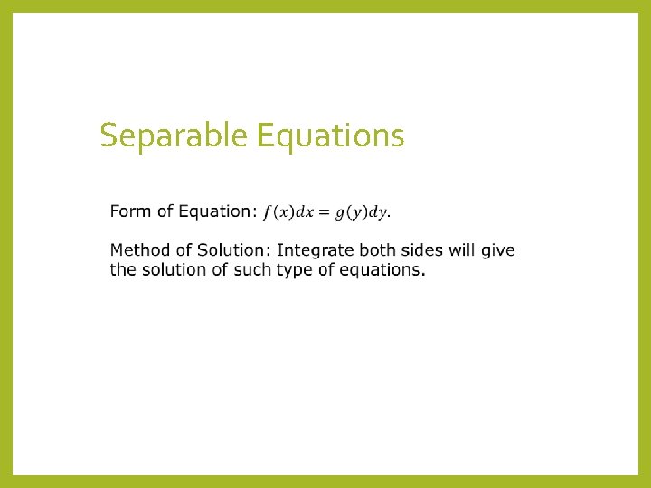
Separable Equations
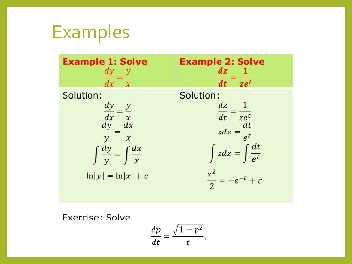
Examples
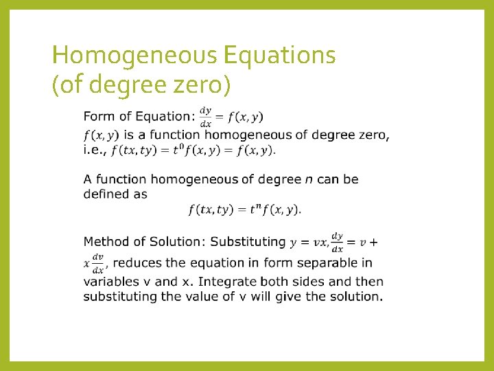
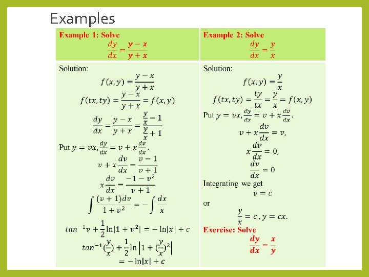
Homogeneous Equations (of degree zero)
Examples
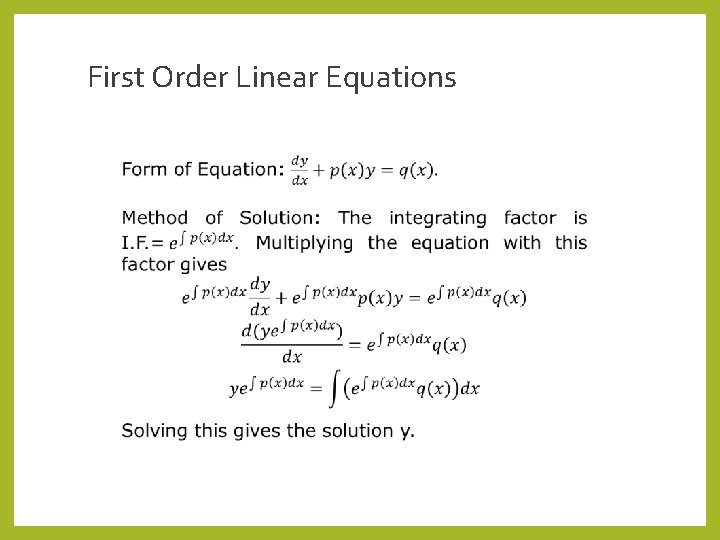
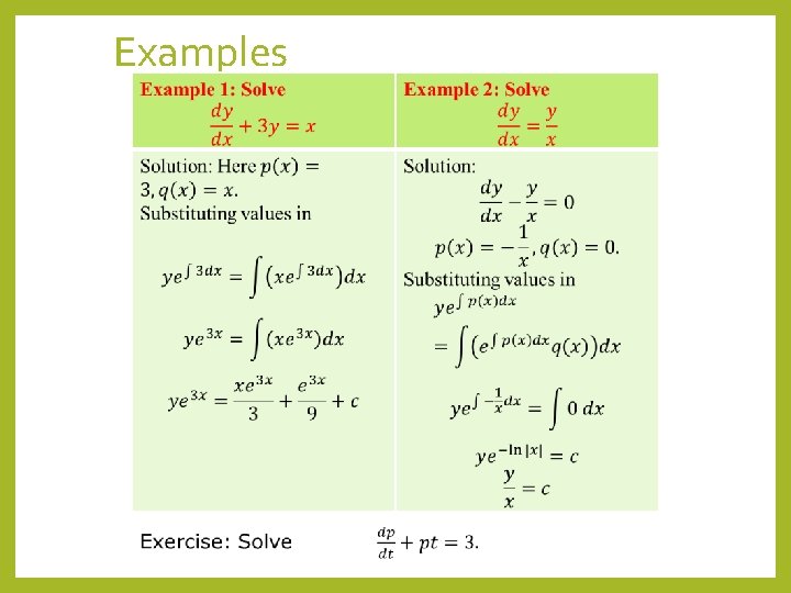
First Order Linear Equations
Examples
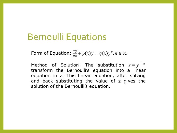
Bernoulli Equations
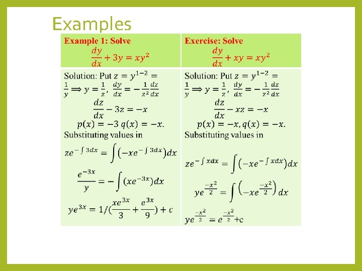
Examples
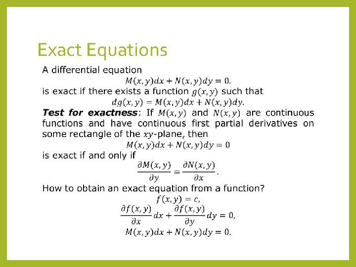
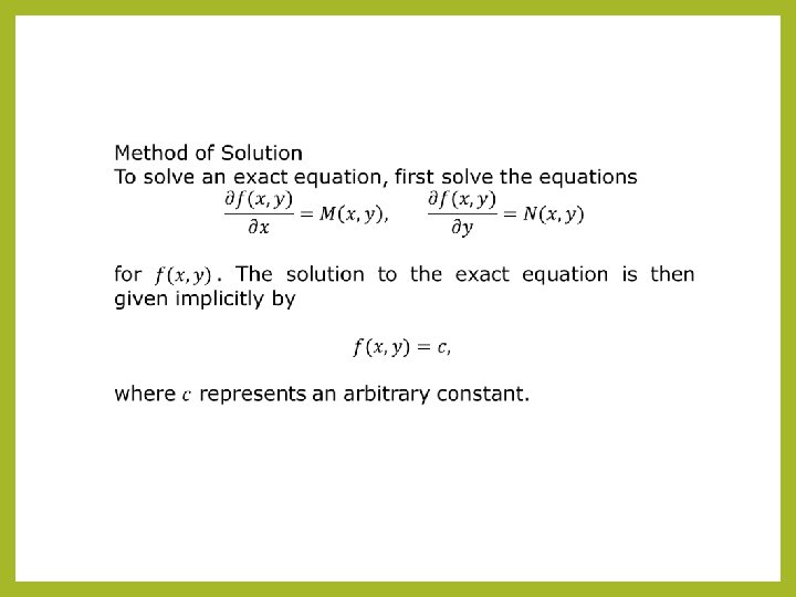
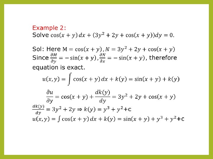
Exact Equations
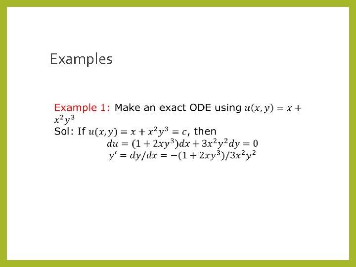
Examples
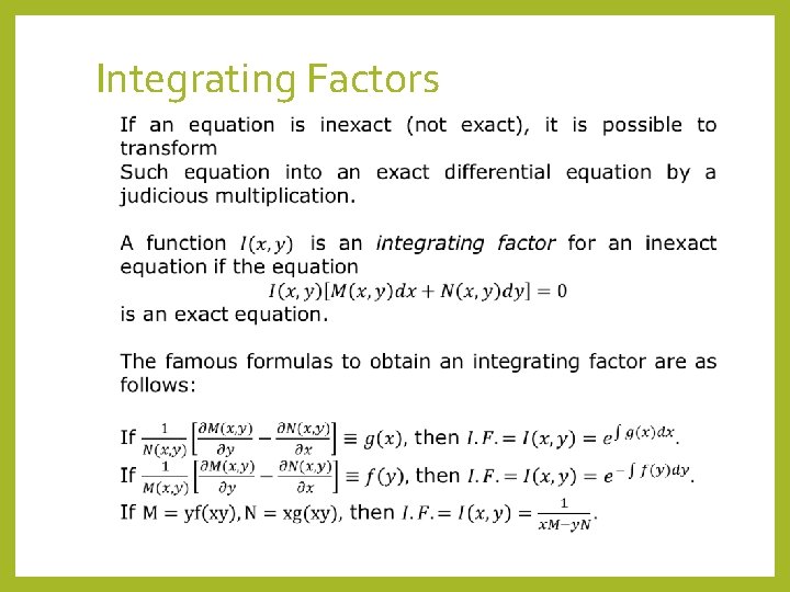
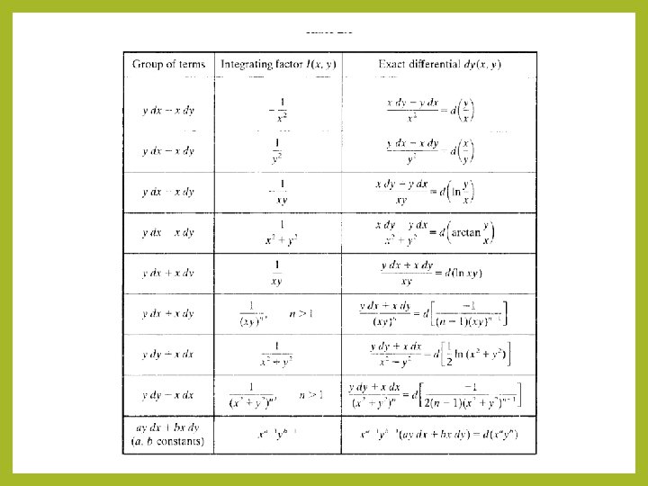
Integrating Factors
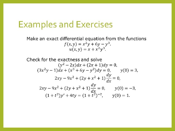
Examples and Exercises
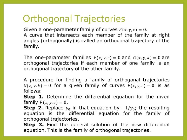
Orthogonal Trajectories
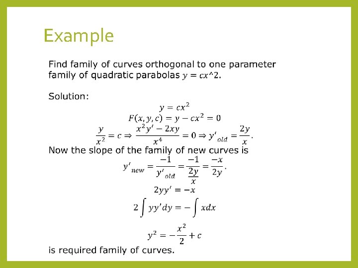
Example
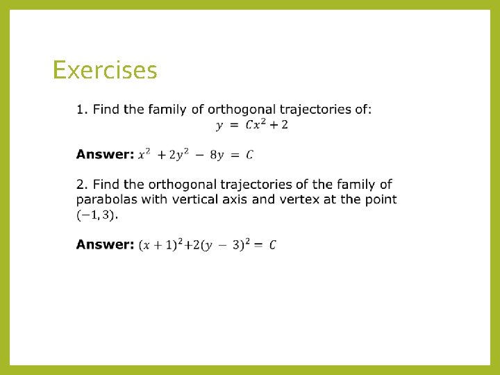
Exercises
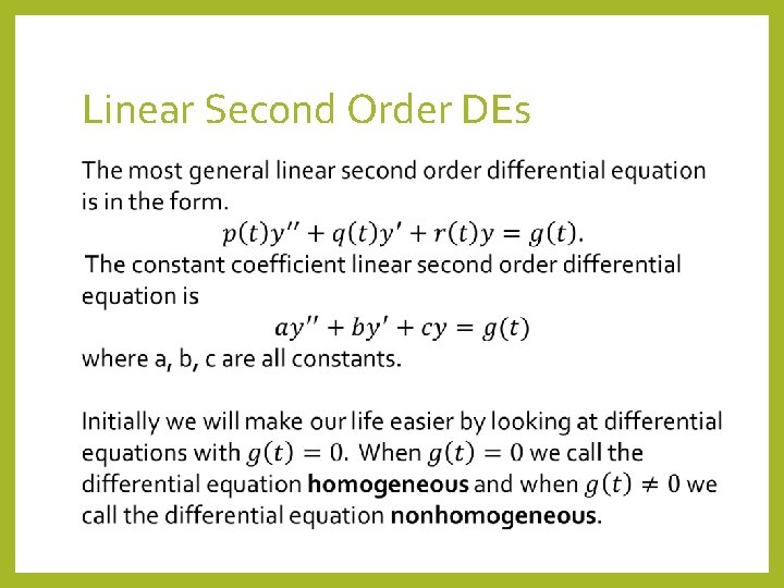
Linear Second Order DEs
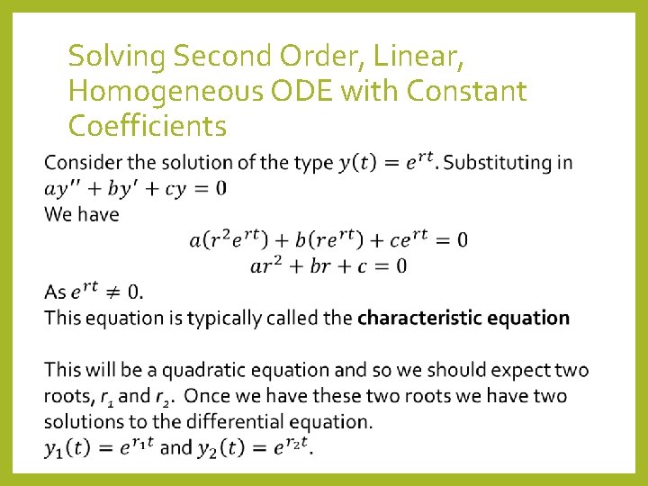
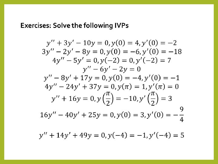
Solving Second Order, Linear, Homogeneous ODE with Constant Coefficients
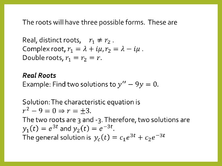
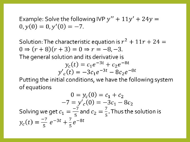
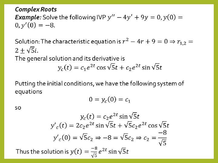
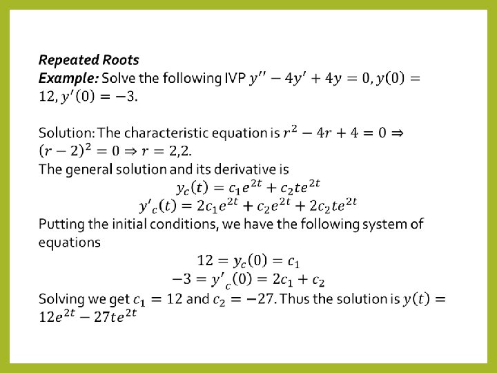
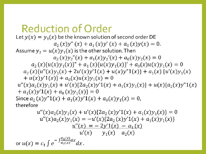
Reduction of Order

Examples and Exercises
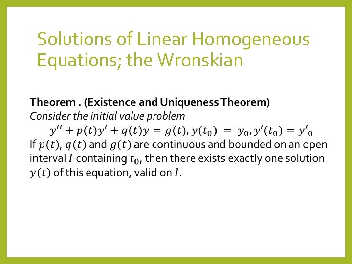
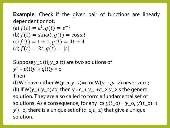
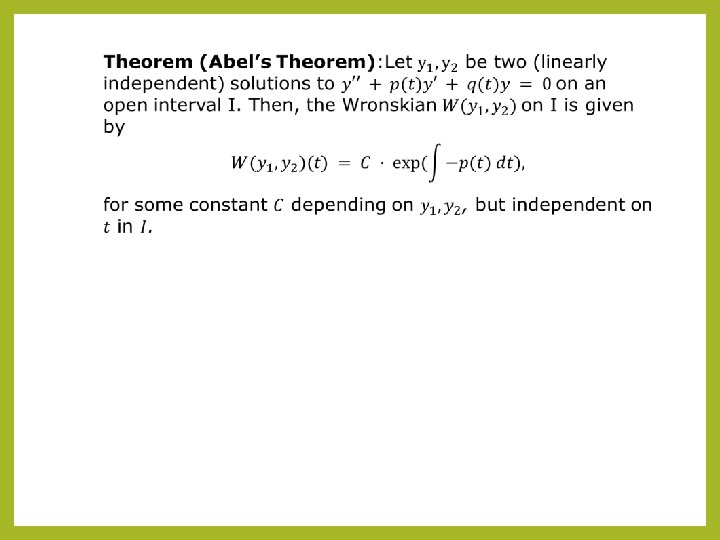
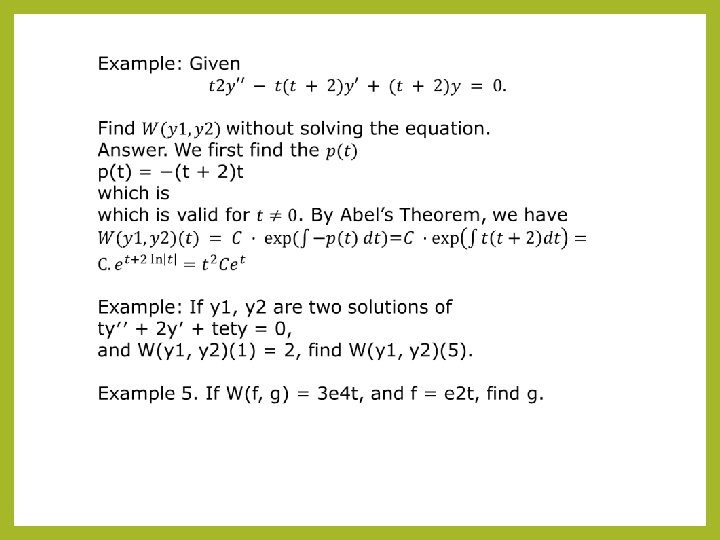
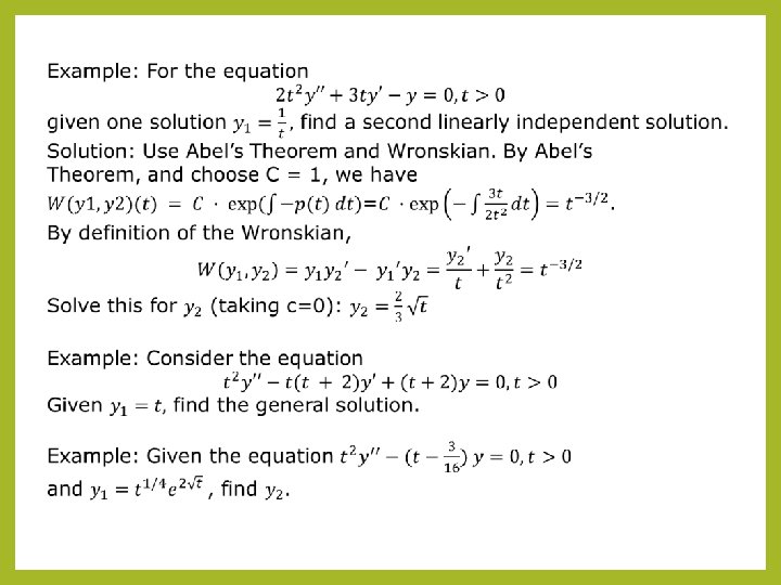
Solutions of Linear Homogeneous Equations; the Wronskian

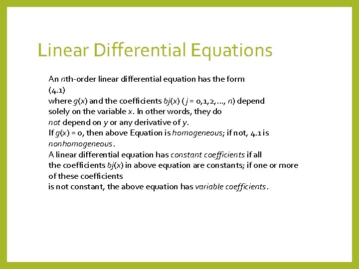
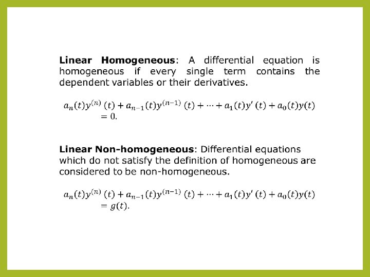
Linear Differential Equations An nth-order linear differential equation has the form (4. 1) where g(x) and the coefficients bj(x) ( j = 0, 1, 2, . . . , n) depend solely on the variable x. In other words, they do not depend on y or any derivative of y. If g(x) = 0, then above Equation is homogeneous; if not, 4. 1 is nonhomogeneous. A linear differential equation has constant coefficients if all the coefficients bj(x) in above equation are constants; if one or more of these coefficients is not constant, the above equation has variable coefficients.
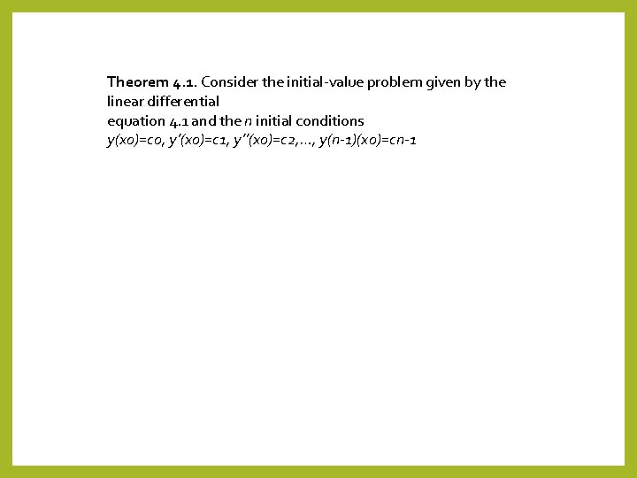
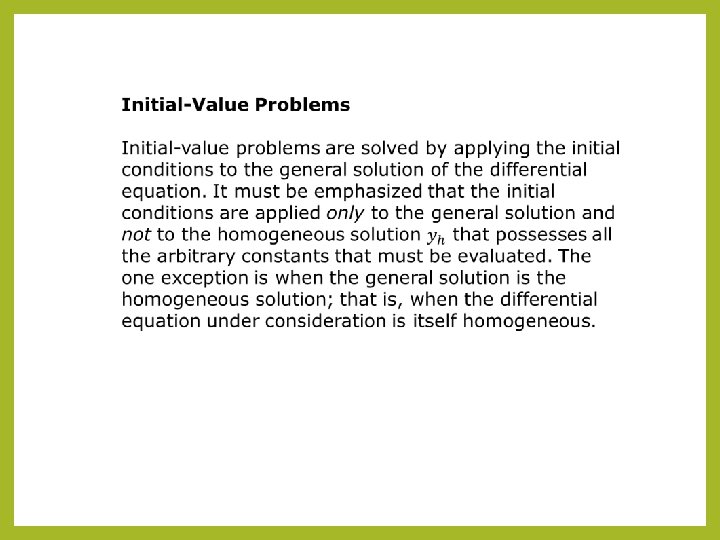
Theorem 4. 1. Consider the initial-value problem given by the linear differential equation 4. 1 and the n initial conditions y(x 0)=c 0, y’(x 0)=c 1, y’’(x 0)=c 2, …, y(n-1)(x 0)=cn-1
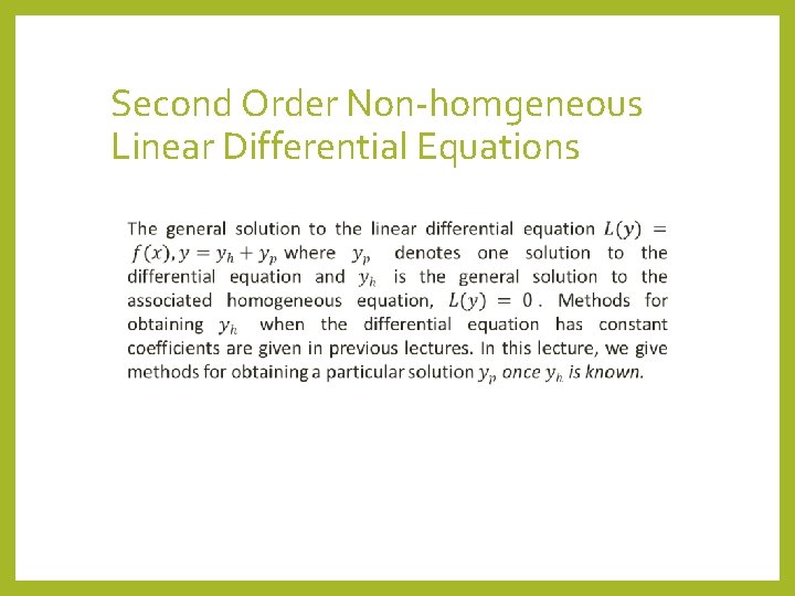
Second Order Non-homgeneous Linear Differential Equations
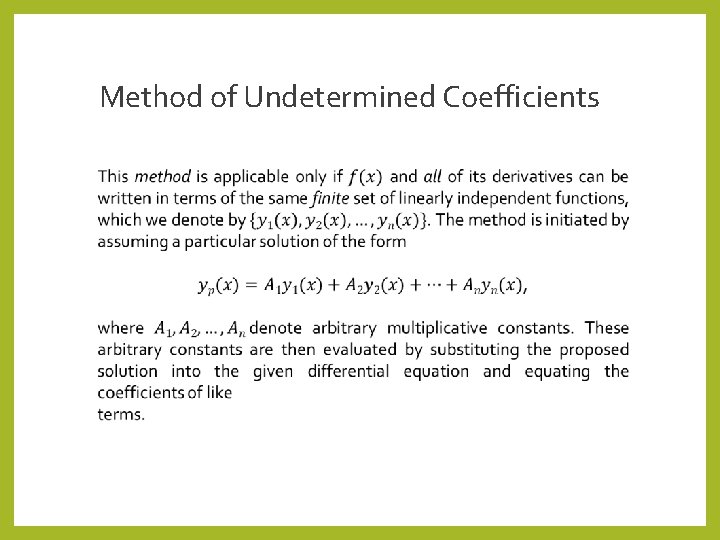
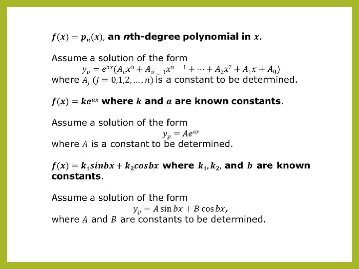
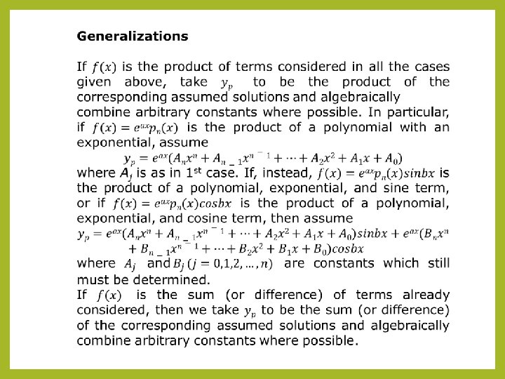
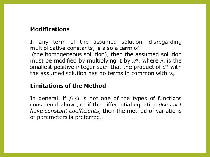
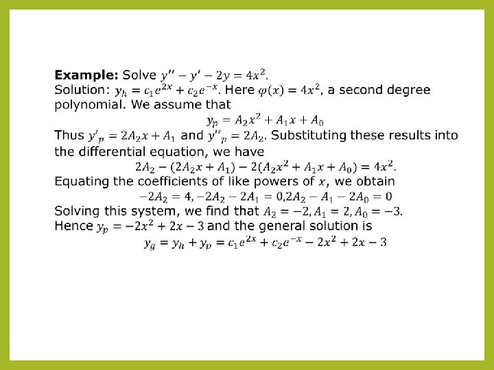
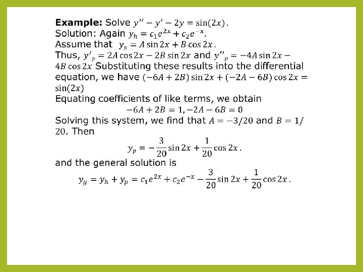
Method of Undetermined Coefficients
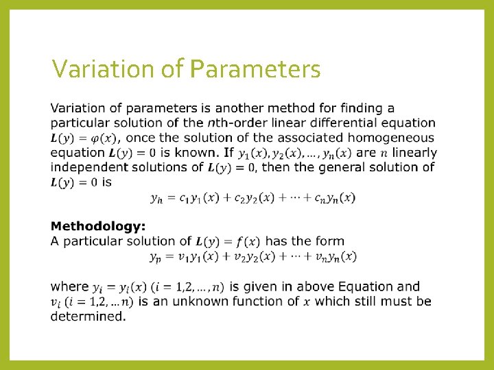
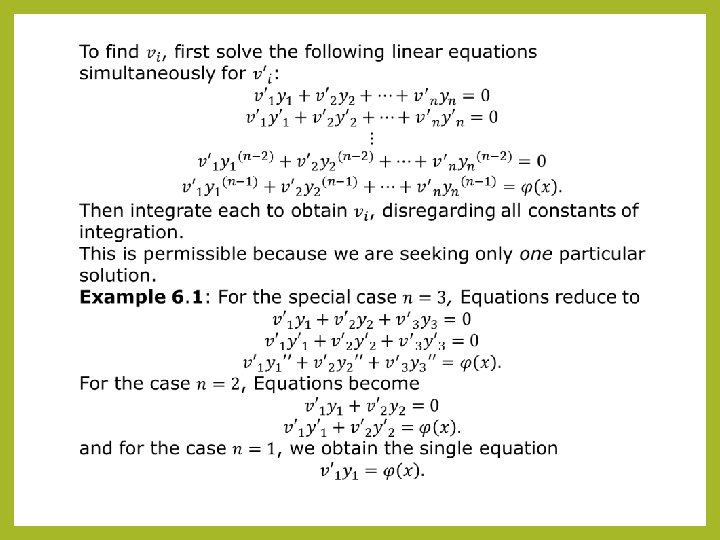
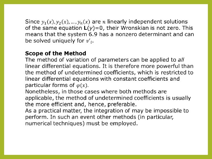
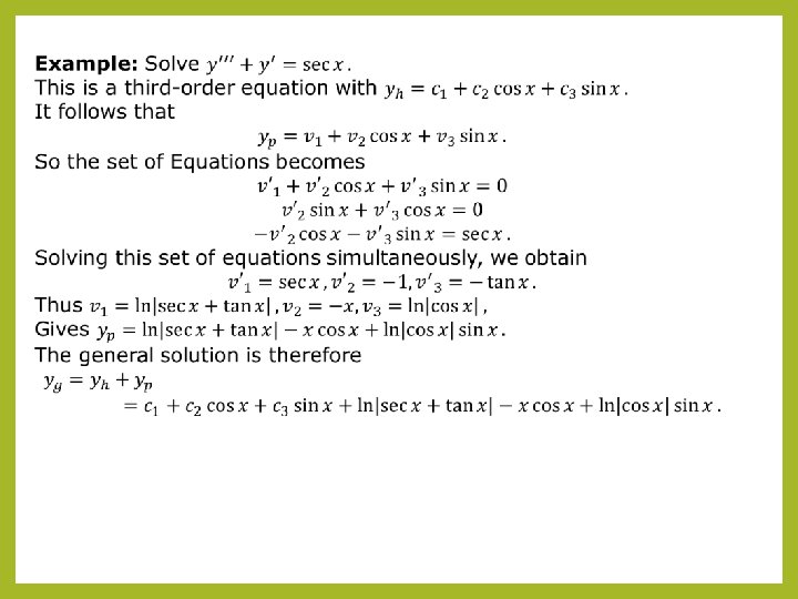
Variation of Parameters
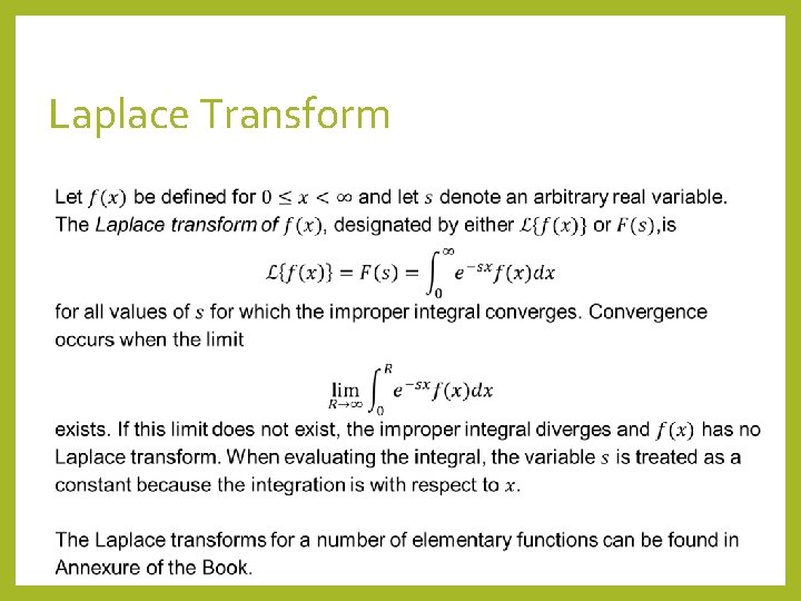
Laplace Transform

Properties of Laplace Transforms
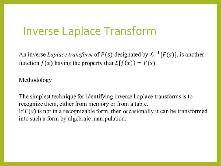
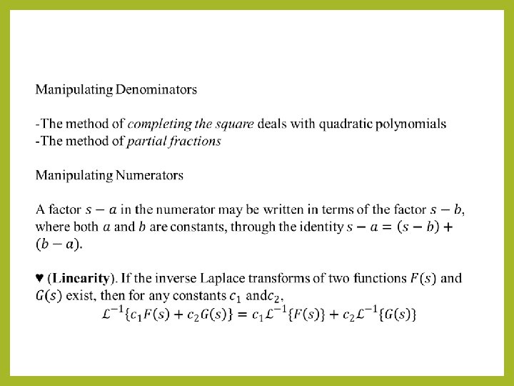
Inverse Laplace Transform
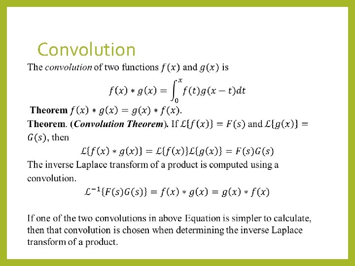
Convolution
- Slides: 66