ENGG 2013 Unit 22 Modeling by Differential Equations

ENGG 2013 Unit 22 Modeling by Differential Equations Apr, 2011.

FREE FALLING BODY kshum 2

Height, velocity and acceleration • Parabola y = – 5 t 2+15 v = – 10 t a = – 10 kshum 3

Newton’s law of motion Assume no air friction • F = ma – Force = mass acceleration – a = y’’(t) • F = mg – Gravitational Force is proportional to the mass, the proportionality constant g – 10 ms-2. y’’(t) = g kshum 4

Differential equation • A differential equation is an equation which involves derivatives. • Examples: dx/dt = x + 2 t The variable x is a function of time t. d 2 y/dt 2 = t 2 + y 2 The variable y is a function of t. kshum 5

Initial conditions • y(0)=0 • y’(0)=10 y(t) = – 5 t 2+10 t+20 y(t) = – 10 t+10 y’’(t) = – 10 kshum 6

Initial conditions • y(0)= – 5 • y’(0)= – 10 y(t) = – 5(t+1)2 y(t) = – 10 t – 10 y’’(t) = – 10 kshum 7

Variables and parameters • The dependent variable is called the system state, or the phase of the system. The independent variable is usually time. • A constant which does not change with time is called a parameter. • In the example Newton’s law of motion y’’(t) = g – Phase = system state = height of the mass – Independent variable = time – g is parameter. kshum 8

Solutions to a differential equation • A solution is a function which satisfies the given differential equation. • In solving differential equation, the solutions are function of time. • In general, there are many solutions to a given differential equation. We have different solutions for different initial condition. • Deriving a solution is difficult, but checking whether a given function is a solution is easy. y(t) = – 5 t 2+15 is a solution to y’’(t) = – 10 because after differentiating – 5 t 2+15 twice, we get – 10. y(t) = 4 t 2 is not a solution to y’’(t) = – 10 because after differentiating 4 t 2 twice, we get 8, not – 10. kshum 9

General solution • If every solution to a differential equation can be obtained from a family of solutions f(t, c 1, c 2, c 3, …, cn) by choosing the constants c 1, c 2, c 3, …, cn appropriately, then we say that f(t, c 1, c 2, c 3, …, cn) is a general solution. kshum 10

General solution to y’’(t) = -10 • For this simple example, just integrate two times. • Integrate both sides of y’’(t) = – 10 y’(t) = – 10 t+c 1 • Integrate both sides of y’(t) = – 10+c 1 y(t) = – 5 t 2+c 1 t+c 2 (general solution) • The constants c 1 and c 2 can be obtained from the initial conditions. kshum 11

FIRST-ORDER DIFFERENTIAL EQUATION kshum 12

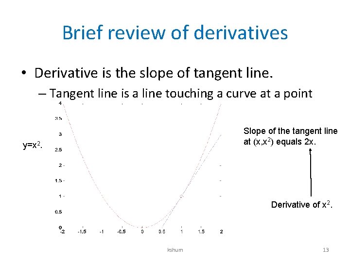
Brief review of derivatives • Derivative is the slope of tangent line. – Tangent line is a line touching a curve at a point Slope of the tangent line at (x, x 2) equals 2 x. y=x 2. Derivative of x 2. kshum 13

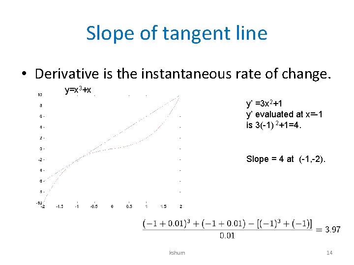
Slope of tangent line • Derivative is the instantaneous rate of change. y=x 3+x y’ =3 x 2+1 y’ evaluated at x=-1 is 3(-1) 2+1=4. Slope = 4 at (-1, -2). kshum 14

First-order differential equation • No second or higher derivative, for example dx/dt = a function of x and t • First-order derivative defines slope. • Example General solution kshum constant 15

An illustration • If an initial condition is given, then we can solve for the constant C. • Suppose that x(0) = 2. C=3. kshum 16

Zoom in at (1, 6. 1548) Line segment with slope -1+e 1=7. 1548. kshum 17

Zoom in at (2, 19. 1672) Line segment with slope – 1 + 3 e 2=21. 1672 kshum 18

Direction field or slope field • A graphical method for solving differential equation. • Systematically evaluate f(x, t) on a grid on points. • On a grid point (t, x), draw a short line segment with slope f(x, t). • A solution must follow the flow pattern. kshum 19

Direction Field for x’=x+t Sample solution for x(0)=2 Each grid point (t, x) is associated with a line segment with slope x+t. kshum 20

Newton’s law of cooling • Imagine a can of coffee in an air-conditioned room. • The rate of change of the temperature T(t) is directly proportional to the difference between T and the temperature T 0 of the environment. • Rate of change in temperature is directly proportional to (T – T 0). – k is a positive constant. – T > T 0, T decreases with rate k (T – T 0). – T < T 0, T increases with rate k (T 0 – T). d. T/dt = – k (T – T 0) kshum (k>0) 21

Rate of change in temperature d. T/dt = – 0. 2 (T – 23) T T 0 T

Direction field d. T/dt = – 0. 2 (T – 23)

Sample solutions d. T/dt = – 0. 2 (T – 23) Some typical solution paths, corresponding initial temperature 0, 5, 10, 15, 20, 25, 30, 35, 40, are shown in the graph.

Autonomous DE and Phase line • Autonomous DE: x’(t) = a function of x only. – no independent variable on the R. H. S. • For autonomous DE, we can understand the system via the phase line. d. T/dt = – k (T– T 0) Phase line T T 0 Critical point at T 0 Stable equilibrium (k>0) T

Direction field for x’=2 x(1 -x) Slopes are zero on these two critical lines. The pattern is the same on every vertical line. kshum 26

Phase line for x’=2 x(1 -x) Without solving the differential equation explicitly, we know that the solution x(t) converges to 1 if it starts at positive x(0), but diverges to negative infinity if it starts at negative x(0). Unstable equilibrium Stable equilibrium Phase line x 0 x 1 x Critical points at x=0 and x=1 kshum 27

Main concepts • Independent variable, dependent variable and parameters • Initial conditions • General solution • Direction field • Autonomous differential equations. – Phase line • Equilibrium – Stable and unstable