ENDMEMBER MIXING ANALYSIS PRINCIPLES AND EXAMPLES Fengjing Liu

END-MEMBER MIXING ANALYSIS: PRINCIPLES AND EXAMPLES Fengjing Liu University of California, Merced

OUTLINES OF LECTURE This tutorial focuses on mathematical procedures, rather than theories, though principles are still addressed where necessary. • MIXING MODEL – Two components using a single tracer – Three components using a pair of tracers – Exercises • PCA • END-MEMBER MIXING ANALYSIS (EMMA) – Principle – Mathematical Procedures

PART 1: OVERVIEW OF HYDROLOGIC MIXING MODELS • • • Review of 2 -Component Mixing Model Assumptions of Mixing Model 3 -Component Mixing Model Generalization of Mixing Models Exercises

MIXING MODEL: 2 COMPONENTS • One Conservative Tracer • Mass Balance Equations for Water and Tracer

ASSUMPTIONS FOR MIXING MODEL • Tracers are conservative (no chemical reactions); • All components have significantly different concentrations for at least one tracer; • Tracer concentrations in all components are temporally constant or their variations are known; • Tracer concentrations in all components are spatially constant or treated as different components; • Unmeasured components have same tracer concentrations or don’t contribute significantly.

MIXING MODEL: 3 COMPONENTS (with Discharge) Simultaneous Equations Solutions • Two Conservative Tracers • Mass Balance Equations for Water and Tracers Q - Discharge C - Tracer Concentration Subscripts - # Components Superscripts - # Tracers

MIXING MODEL: 3 COMPONENTS (Using Discharge Fractions) Simultaneous Equations Solutions • Two Conservative Tracers • Mass Balance Equations for Water and Tracers f - Discharge Fraction C - Tracer Concentration Subscripts - # Components Superscripts - # Tracers

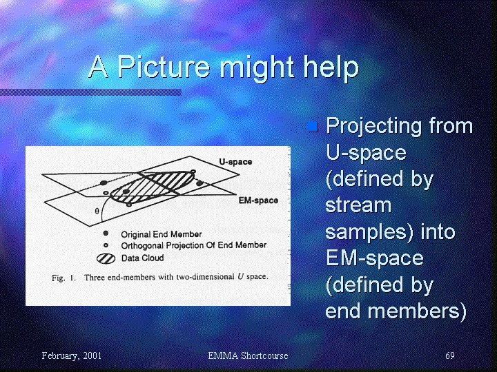
MIXING MODEL: Geometrical Perspective • For a 2 -tracer 3 -component model, for instance, the mixing subspaces are defined by two tracers. • If plotted, the 3 components should be vertices of a triangle and all streamflow samples should be bound by the triangle. • If not well bound, either tracers are not conservative or components are not well characterized. • fx can be sought geometrically, but more difficult than algebraically.

MIXING MODEL: Generalization Using Matrices • One tracer for 2 components and two tracers for 3 components • N tracers for N+1 components? -- Yes • However, solutions would be too difficult for more than 3 components • So, matrix operation is necessary Simultaneous Equations Where Solutions Note: • Cx-1 is the inverse matrix of Cx • This procedure can be generalized to N tracers for N+1 components

MATHEMATICAL UNCERTAINTY Expression of two-tracer three-component mixing model Determinant of coefficients Solutions

MATHEMATICAL UNCERTAINTY Uncertainty for three component model based on a Gaussian error propagation [Genereux, 1998]: For a twocomponent model: W = standard deviation f = fractions of flow components C = tracer concentrations in flow components

SOLUTION FOR OUTLIERS • A, B, and C are 3 endmembers; • D is an outlier of streamflow sample; • E is the projected point of D to line AB; • a, b, d, x, and y represent distance of two points; • We will use Pythagorean theorem to resolve it. • The basic rule is to force fc = 0, f. A and f. B are calculated below [Liu et al. , 2004]:

THOUGHTS OF TRADITIONAL MIXING MODELS • Are results consistent b/w the models using SO 42 - and 18 O versus Si and 18 O? • Why? • Is it difficult to solve a two-tracer threecomponent mixing model? • Unclear if you get the right result for the right reasons – Because may not meet all the assumptions

PART 2: PCA • • PCA Overview Steps Eigenvalues and Eigenvectors Examples

Principal Component Analysis (PCA) is the heart of EMMA • PCA is a multivariate method of analysis and has been used widely with large multidimensional data sets. • The use of PCA allows the number of variables in a multivariate data set to be reduced, • whilst retaining as much as possible of the variation present in the data set.

PCA Overview • Essentially, you are collapsing a lot of variables (columns) with numerous measurements (rows) into just a few principal components

How does PCA do this? • • • Essentially, a set of correlated variables are transformed into a set of uncorrelated variables which are ordered by reducing variability. The uncorrelated variables are linear combinations of the original variables, and the last of these variables can be removed with minimum loss of real data. The transformed data are rotated such that maximum variabilities are projected onto the PCA axes.

Steps • First, we normalize the data so the mean is 0 and the standard deviation is one; • Next, we construct a correlation or covariance matrix; • Then we perform PCA analysis

Lets look at a data set with two columns after normalizing the data

The PCA is then performed. The red line represents the direction of the first principal component and the green is the second. Note how the first principal component lies along the line of greatest variation, and the second lies perpendicular to it.

Rotate data so the PC’s lie along the axes We do this by multiplying the original data-set by the principal components (let a software package do this)

Lets step through PCA analysis using water quality data from wells and springs

Normal water quality data Columns are the variables (n = 7) Rows are the observations. Here the rows are different sites. Often the rows are repeated observations of the same variables from the same site

Pearson’s correlation table • Produces a matrix with equal rows and columns • All the data are normalized. • Ca, Mg, Na, Fe, and Zn highly correlated • 18 O is inversely correlated to them • Ar is not significantly correlated with anything

Calculate eigenvectors and eigenvalues • Eigenvectors of transformations are vectors which are either left unaffected or simply multiplied by a scale factor after the transformation. • An eigenvector's eigenvalue is the scale factor that it has been multiplied by.

Eigenvalues and Factors • Eigenvalues reflect the quality of the projection from the N-dimensional initial table (N=7 in this example) to a lower number of dimensions. • Each eigenvalue corresponds to a factor, and each factor to one dimension. • A factor is a linear combination of the initial variables, and all the factors are uncorrelated (r=0). • The eigenvalues and the corresponding factors are sorted by descending order of how much of the initial variability they represent (converted to %).

Calculate eigenvalues and factors In this example, we can see that the first eigenvalue equals 5. 829 and represents 83% of the total variability. This means that if we represent the data on only one axis, we will still be able to see 83% of the total variability of the data.

Eigenvalues plotted as percent of total variance in our data The first two factors explain 98% of the variance

Biplot helps visualize eigenvalues

Interpretation of the biplot • Close to each other, they are significantly positively correlated (r close to 1); • If they are orthogonal, they are not correlated (r close to 0); • If they are on the opposite side of the center, then they are significantly negatively correlated (r close to -1). • When the variables are close to the center, it means that some information is carried on other axes, and that any interpretation might be hazardous.

Our data set • Ca, Na, Mg, Fe, and Zn all plot together , suggesting a geochemical weathering signal • 18 O plots on the opposite side of the center, suggesting a strong negative correlation • Ar plots orthogonal to the first axis, suggesting a second factor that might be related to pollution

Plot the eigenvectors Wells Springs

Interpretation • Wells plot together and springs plot together • Wells and spring both plot primarily on the first axis, suggesting a common geochemical weathering signal • Springs plot on a negative position along the first axis, suggesting a different recharge source than the wells • Sites that plot on the positive second axis have a pollution signal superimposed on the geochemical signal

PCA software tools • XLSTAT • Matlab – Public domain code • Hornberger book • IDL

PART 3: EMMA • EMMA overview • Procedures for EMMA • Examples

END-MEMBER MIXING ANALYSIS • EMMA used for null hypothesis test to reject end-members that are not significantly contributing to the targeted stream in terms of water quantity; • Uses more tracers than components; • Decides number of end-members; • Quantitatively select end-members; • Quantitatively evaluate results of EMMA.

EMMA PROCEDURES • Identification of Conservative Tracers & Number of End. Members - Bivariate solute-solute plots to screen data; • PCA Performance - Derive eigenvalues and eigenvectors; • Number of End-members – Check using eigenvalues • Orthogonal Projection - Use eigenvectors to project chemistry of streamflow and end-members; • Screen End-Members - Calculate Euclidean distance of endmembers between their original values and S-space projections; • Hydrograph Separation - Use orthogonal projections and generalized equations for mixing model to get solutions! • Validation of Mixing Model - Predict streamflow chemistry using results of hydrograph separation and original end-member concentrations.

Identify conservative tracers & # of end-members • Look familiar? • This is the same diagram used for geometrical definition of mixing model (components changed to end-members); • Generate all plots for all pair-wise combinations of tracers; • The simple rule to identify conservative tracers & # of endmembers is to see if streamflow samples can be bound by a polygon formed by potential end-members or scatter around a line defined by two end-members; • Be aware of outliers and curvature which may indicate chemical reactions!

APPLICATION IN GREEN LAKES VALLEY: NWT LTER RESEARCH SITE Green Lake 4 Sample Collection • Stream water weekly grab samples • Snowmelt - snow lysimeter • Soil water - zero tension lysimeter • Talus water – biweekly to monthly Sample Analysis • 18 O and major solutes

S T R E A M C H E MI S T R Y A ND DI S CHA RG E Solutes vary by 2 -3 x Discharge varies by 10 x

Identify conservative tracers & # of end-members

Eigenvectors and PCA Components

APPLICATION OF EIGENVALUES • Eigenvalues can be used to infer the number of endmembers that should be used in EMMA. How? • Sum up all eigenvalues; • Calculate percentage of each eigenvalue in the total eigenvalue; • The percentage should decrease from PCA component 1 to p (remember p is the number of solutes used in PCA); • How many eigenvalues can be added up to 90% (somewhat subjective! No objective criteria for this!)? Let this number be m, which means the number of PCA components should be retained (sometimes called # of mixing spaces); • (m +1) is equal to # of end-members we use in EMMA.

Mixing Diagrams Using PCA Components • Plot a scatter plot for streamflow samples and end-members using the first and second PCA projections; • Eligible end-members should be vertices of a polygon (a line if m = 1, a triangle if m = 2, and a quadrilateral if m = 3) and should bind streamflow samples in a convex sense;

SCREEN END-MEMEBRS Algebraically • Calculate the Euclidean distance between original chemistry and projections for each solute using the equations below: • j represent each solute and bj is the original solute value Those steps should lead to identification of eligible end-members!

HYDROGRAPH SEPARATION • Use the retained PCA projections from streamflow and endmembers to derive flowpath solutions! • So, mathematically, this is the same as a general mixing model rather than the over-determined situation. U with superscripts are the principal components. Subscripts are the different end-members.

FLOWPATHS: EMMA Liu et al, 04, WRR

EVALUATE THE RESULTS • Multiply results of hydrograph separation (usually fractions) by original solute concentrations of endmembers to reproduce streamflow chemistry for conservative solutes; • Comparison of the prediction with the observation can lead to a test of mixing model.

TEFLON MYTH DEBUNKED Shallow groundwater system • Almost 50% of flow on the rising limb is “old” groundwater: baseflow and talus • Up to 80% of water on the recession limb is groundwater • Most of “new” water from snow melt infiltrates into the subsurface • Geographically isolated source waters can be identified

REFERENCES Christophersen, N. , C. Neal, R. P. Hooper, R. D. Vogt, and S. Andersen, Modeling stream water chemistry as a mixture of soil water end-members – a step towards second-generation acidification models, Journal of Hydrology, 116, 307 -320, 1990. • Christophersen, N. and R. P. Hooper, Multivariate analysis of stream water chemical data: the use of principal components analysis for the end-member mixing problem, Water Resources Research, 28(1), 99 -107, 1992. • Hooper, R. P. , N. Christophersen, and N. E. Peters, Modeling stream water chemistry as a mixture of soil water end-members – an application to the Panola mountain catchment, Georgia, U. S. A. , Journal of Hydrology, 116, 321 -343, 1990. • Hooper, R. P, Diagnostic tools for mixing models of stream water chemistry, Water Resources Research, 39(3), 1055, doi: 10. 1029/2002 WR 001528, 2003. • Burns, D. , Mc. Donnell JJ, Hooper RP, et al. Quantifying contributions to storm runoff through end-member mixing analysis and hydrologic measurements at the Panola Mountain Research Watershed (Georgia, USA) HYDROLOGICAL PROCESSES 15 (10): 1903 -1924 JUL 2001 • Liu, F. , M. Williams, and N. Caine. Source waters and flowpaths in a seasonally snow-covered catchment, Colorado Front Range, USA, Water Resources Research, Vol 40, W 09401, 2004.