Ence 627 Decision Analysis for Engineering Project Portfolio

Ence 627 Decision Analysis for Engineering Project Portfolio Selection: “Optimal Budgeting of Projects Under Uncertainty” Javier Ordóñez

Overview “Optimal Budgeting of Projects Under Uncertainty” n n n 4 Projects to be allocated in 3 years Projects’ costs are uncertain No more than 2 projects can be selected per year Initial budget is also uncertain The policy of the budget use says that as much as the budget should be used (minimize residual)

How do I decide what project to fund and when? Stochastic Dynamic Programming: n n SDP is a framework for modeling optimization problems that involve uncertainty. The goal is to find a policy which is feasible for all (or almost all) the possible data instances and maximizes/minimizes the expectation of some function of the decision and the random variables. SDP takes advantage of the fact that probability distributions are known or can be estimated. Recourse: ability to take corrective action after a random event has taken place

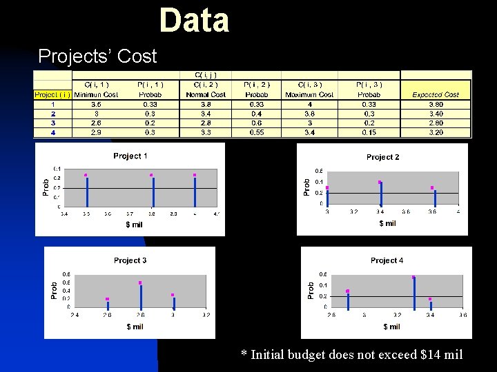
Data Projects’ Cost * Initial budget does not exceed $14 mil

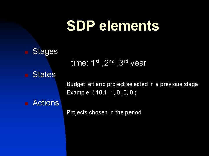
SDP elements n Stages time: 1 st , 2 nd , 3 rd year n States Budget left and project selected in a previous stage Example: ( 10. 1, 1, 0, 0, 0 ) n Actions Projects chosen in the period

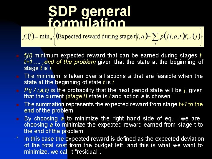
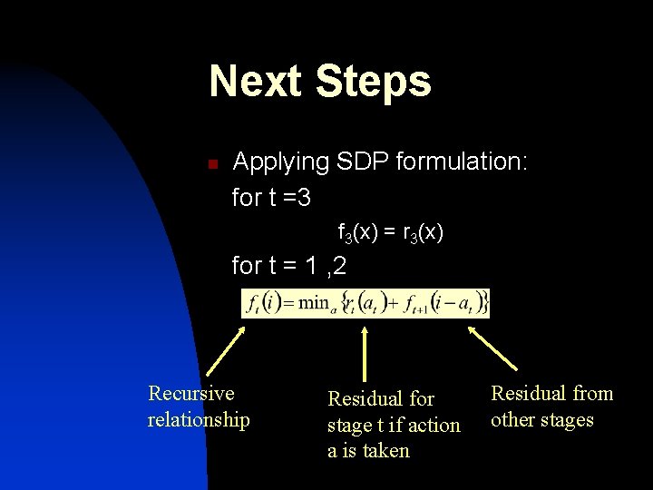
SDP general formulation ft(i) minimum expected reward that can be earned during stages t, t+1…. , end of the problem given that the state at the beginning of stage t is i n The minimum is taken over all actions a that are feasible when the state at the beginning of state t is i n P(j / i, a, t) is the probability that the next period state will be j, given that the current (stage t) state is i and action a is chosen. n The summation represents the expected reward from stage t+1 to the end of the problem n By choosing a to minimize the right hand side of eq. , we are choosing a to minimize the expected reward earned from stage t to the end of the problem * In this case the expected reward is defined as the expected deviation of the total cost from the budget left, and this is what we want to minimize, we call it “residual”. n

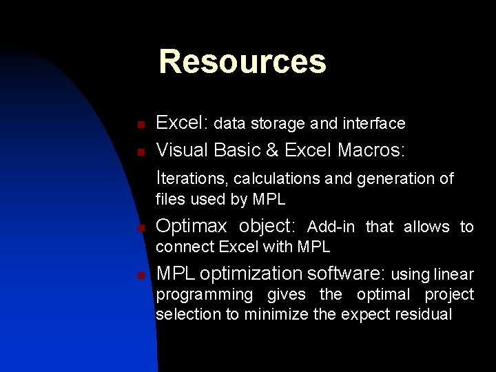
Resources n n Excel: data storage and interface Visual Basic & Excel Macros: Iterations, calculations and generation of files used by MPL n Optimax object: Add-in that allows to connect Excel with MPL n MPL optimization software: using linear programming gives the optimal project selection to minimize the expect residual

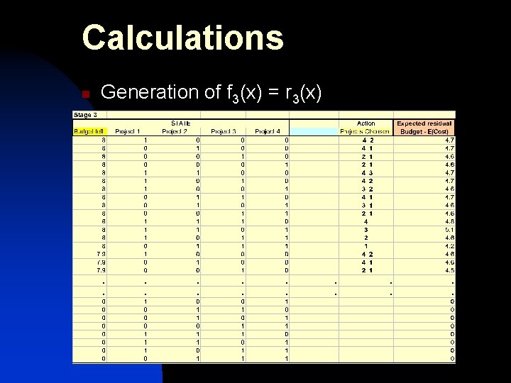
Calculations n n Generation of f 3(x) = r 3(x) What This Means Add a strong statement that summarizes how you feel or think about this topic Summarize key points you want your audience to remember

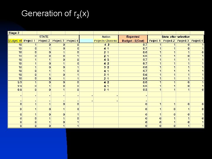
Generation of r 2(x)

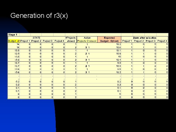
Generation of r 3(x)

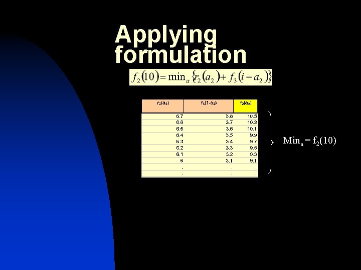
Next Steps n Applying SDP formulation: for t =3 f 3(x) = r 3(x) for t = 1 , 2 Recursive relationship Residual for stage t if action a is taken Residual from other stages

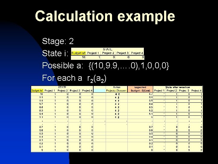
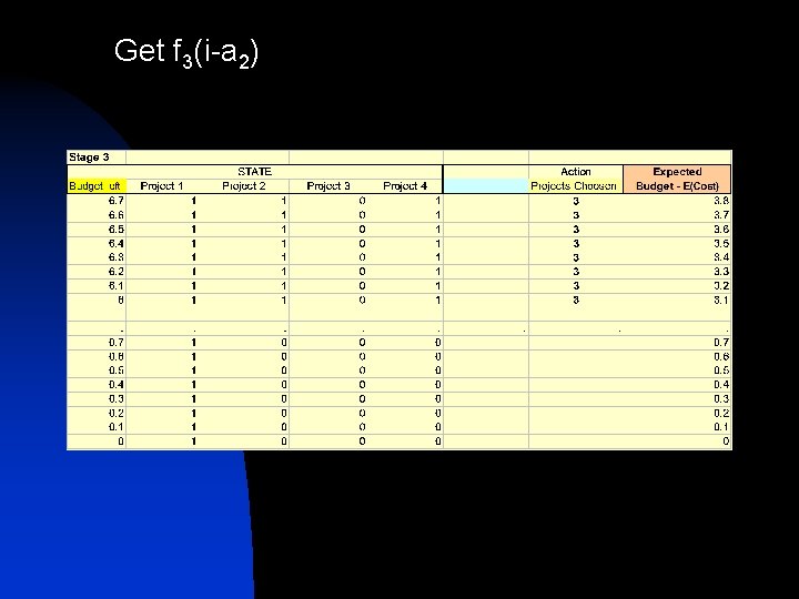
Calculation example Stage: 2 State i: Possible a: {(10, 9. 9, …. 0), 1, 0, 0, 0} For each a r 2(a 2)

Get f 3(i-a 2)

Applying formulation Mina = f 2(10)

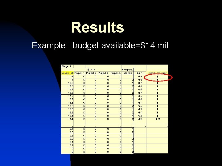
Results Example: budget available=$14 mil

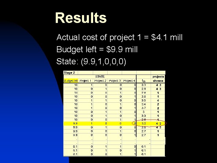
Results Actual cost of project 1 = $4. 1 mill Budget left = $9. 9 mill State: (9. 9, 1, 0, 0, 0)

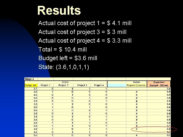
Results Actual cost of project 1 = $ 4. 1 mill Actual cost of project 3 = $ 3 mill Actual cost of project 4 = $ 3. 3 mill Total = $ 10. 4 mill Budget left = $3. 6 mill State: (3. 6, 1, 0, 1, 1)

Model statistics Possible states: 2426 Iterations for possible scenarios: around 300’ 000, 000 Time to run the program 1 h 15

Future work Increase the number of projects Multi-objective optimization: cost & resources Improve program functionality

Questions?