Empirical Testing of Solar Coronal and Solar Wind

Empirical Testing of Solar Coronal and Solar Wind Models Lauren Woolsey University of Maryland - College Park (2011) Mentor: Dr. Leonard Strachan

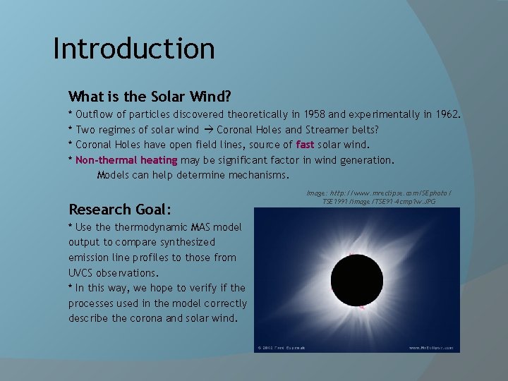
Introduction What is the Solar Wind? * * Outflow of particles discovered theoretically in 1958 and experimentally in 1962. Two regimes of solar wind Coronal Holes and Streamer belts? Coronal Holes have open field lines, source of fast solar wind. Non-thermal heating may be significant factor in wind generation. Models can help determine mechanisms. Research Goal: * Use thermodynamic MAS model output to compare synthesized emission line profiles to those from UVCS observations. * In this way, we hope to verify if the processes used in the model correctly describe the corona and solar wind. Image: http: //www. mreclipse. com/SEphoto/ TSE 1991/image/TSE 91 -4 cmp 1 w. JPG

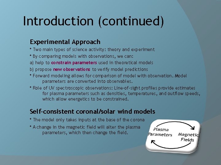
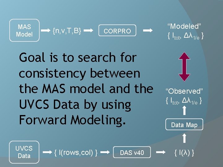
Introduction (continued) Experimental Approach * Two main types of science activity: theory and experiment * By comparing models with observations, we can: a) help to constrain parameters used in theoretical models b) propose new observations to verify model predictions * Forward modeling allows for comparison of model with observation. Model parameters are converted into observables. * Role of UV spectroscopic observations: Line-of-sight profiles provide estimates for plasma parameters such as densities, temperatures, and outflow speeds, which allow energetics to be constrained. Self-consistent coronal/solar wind models * The model only takes inputs at the base of the corona * A change in the magnetic field will alter the plasma parameters, which then change the field.

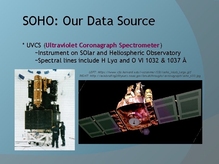
SOHO: Our Data Source * UVCS (Ultraviolet Coronagraph Spectrometer) ~Instrument on SOlar and Heliospheric Observatory ~Spectral lines include H Lyα and O VI 1032 & 1037 Å LEFT: https: //www. cfa. harvard. edu/~scranmer/SSU/soho_inlab_large. gif RIGHT: http: //celebrating 200 years. noaa. gov/breakthroughs/coronagraph/soho_650. jpg

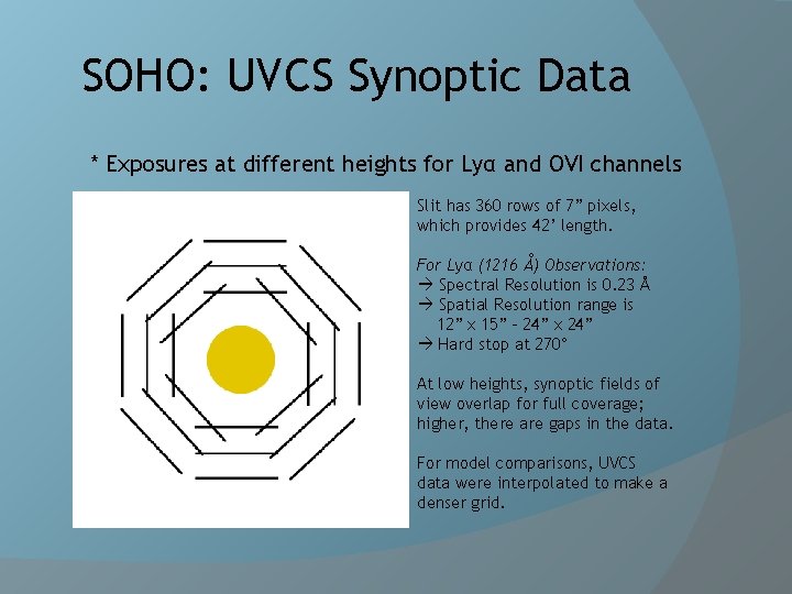
SOHO: UVCS Synoptic Data * Exposures at different heights for Lyα and OVI channels Slit has 360 rows of 7” pixels, which provides 42’ length. For Lyα (1216 Å) Observations: Spectral Resolution is 0. 23 Å Spatial Resolution range is 12” x 15” – 24” x 24” Hard stop at 270° At low heights, synoptic fields of view overlap for full coverage; higher, there are gaps in the data. For model comparisons, UVCS data were interpolated to make a denser grid.

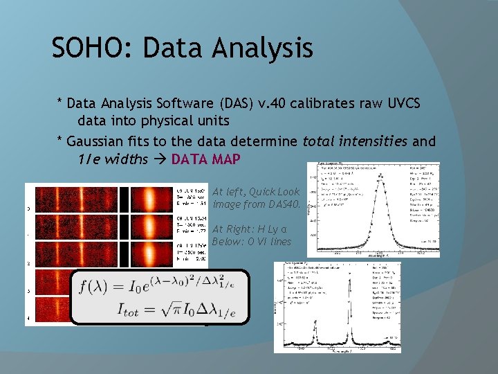
SOHO: Data Analysis * Data Analysis Software (DAS) v. 40 calibrates raw UVCS data into physical units * Gaussian fits to the data determine total intensities and 1/e widths DATA MAP At left, Quick Look image from DAS 40. At Right: H Ly α Below: O VI lines

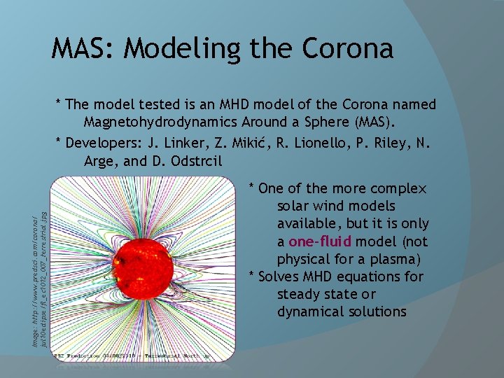
MAS: Modeling the Corona Image: http: //www. predsci. com/corona/ jul 10 eclipse/fl_ec 1012_007_terrestrial. jpg * The model tested is an MHD model of the Corona named Magnetohydrodynamics Around a Sphere (MAS). * Developers: J. Linker, Z. Mikić, R. Lionello, P. Riley, N. Arge, and D. Odstrcil * One of the more complex solar wind models available, but it is only a one-fluid model (not physical for a plasma) * Solves MHD equations for steady state or dynamical solutions

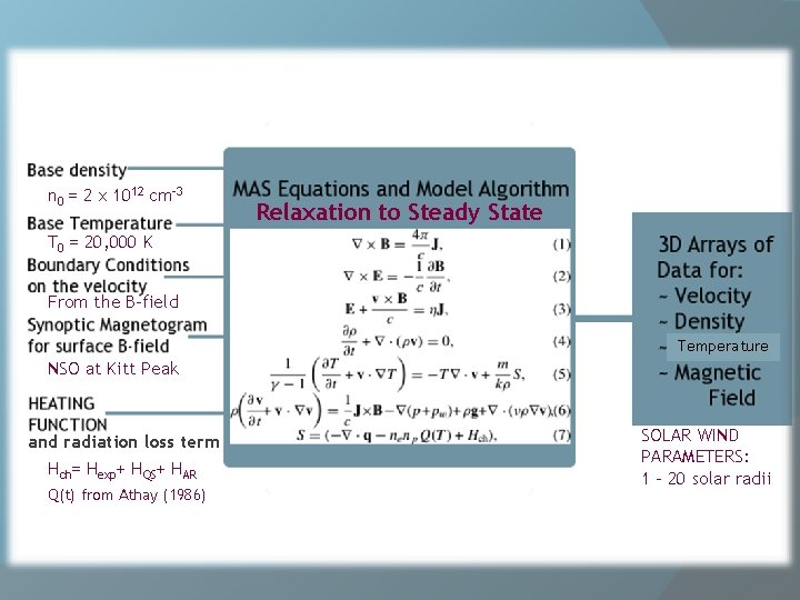
n 0 = 2 x 1012 cm-3 Relaxation to Steady State T 0 = 20, 000 K From the B-field Temperature NSO at Kitt Peak and radiation loss term Hch= Hexp+ HQS+ HAR Q(t) from Athay (1986) SOLAR WIND PARAMETERS: 1 – 20 solar radii

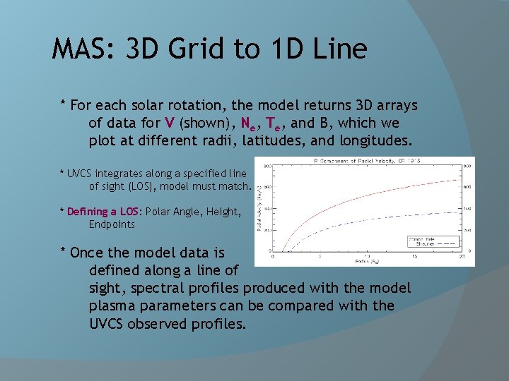
MAS: 3 D Grid to 1 D Line * For each solar rotation, the model returns 3 D arrays of data for V (shown), Ne, Te, and B, which we plot at different radii, latitudes, and longitudes. * UVCS integrates along a specified line of sight (LOS), model must match. * Defining a LOS: Polar Angle, Height, Endpoints * Once the model data is defined along a line of sight, spectral profiles produced with the model plasma parameters can be compared with the UVCS observed profiles.

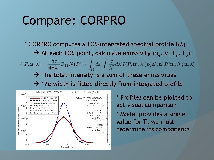
Compare: CORPRO * CORPRO computes a LOS-integrated spectral profile I(λ) At each LOS point, calculate emissivity (ne, v, Te, Tp): The total intensity is a sum of these emissivities 1/e width is fitted directly from integrated profile * Profiles can be plotted to get visual comparison * Model provides a single value for T, we must determine its components

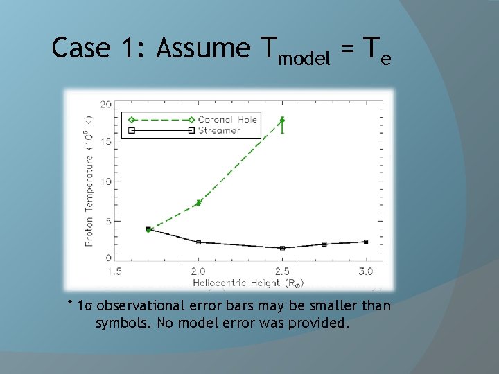
Case 1: Assume Tmodel = Te * Solve Tp by matching Imodel = Iobs * Electron temperature controls ionization fraction N(P) term in total intensity * Proton Temperature is a “kinetic temperature. ” It controls the 1/e width. However, Tp can also affect total intensity through Doppler dimming. * Tp is determined by adjusting the parameter until the modeled intensity matches observed intensity (within data uncertainty) * 1σ observational error bars may be smaller than symbols. No model error was provided.

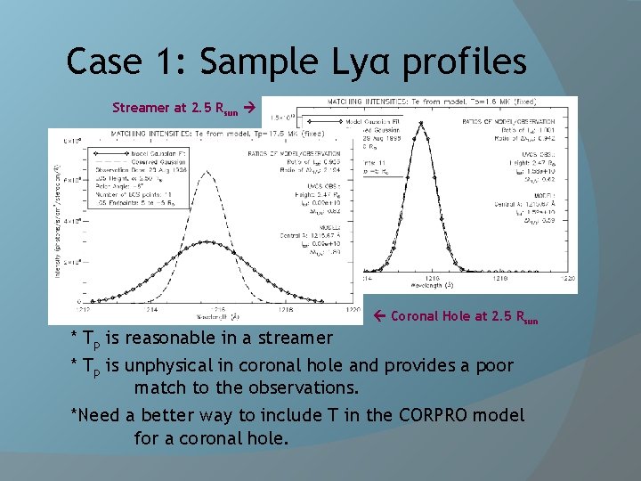
Case 1: Sample Lyα profiles Streamer at 2. 5 Rsun Coronal Hole at 2. 5 Rsun * Tp is reasonable in a streamer * Tp is unphysical in coronal hole and provides a poor match to the observations. *Need a better way to include T in the CORPRO model for a coronal hole.

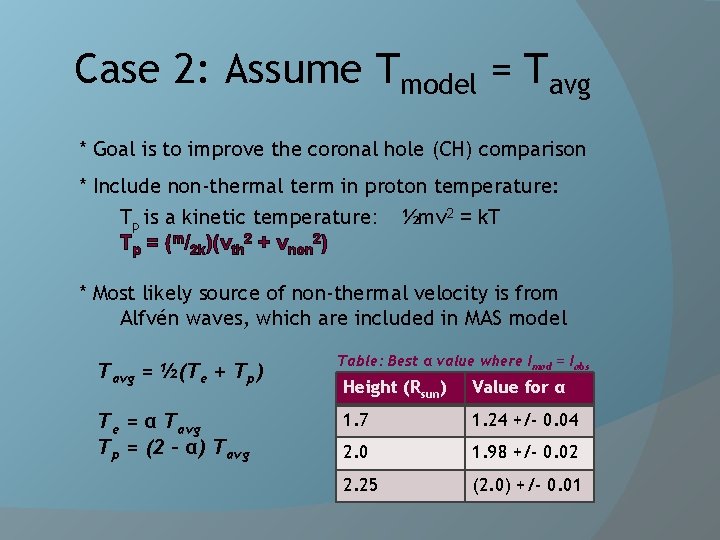
Case 2: Assume Tmodel = Tavg * Goal is to improve the coronal hole (CH) comparison * Include non-thermal term in proton temperature: Tp is a kinetic temperature: ½mv 2 = k. T Tp = (m/2 k)(vth 2 + vnon 2) * Most likely source of non-thermal velocity is from Alfvén waves, which are included in MAS model Tavg = ½(Te + Tp) Te = α Tavg Tp = (2 – α) Tavg Table: Best α value where Imod = Iobs Height (Rsun) Value for α 1. 7 1. 24 +/- 0. 04 2. 0 1. 98 +/- 0. 02 2. 25 (2. 0) +/- 0. 01

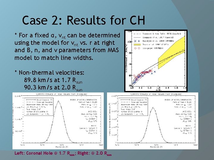
Case 2: Results for CH * For a fixed α, vnt can be determined using the model for vnt vs. r at right and B, n, and v parameters from MAS model to match line widths. * Non-thermal velocities: 89. 8 km/s at 1. 7 Rsun 90. 3 km/s at 2. 0 Rsun Landi & Cranmer (2009) Left: Coronal Hole @ 1. 7 Rsun; Right: @ 2. 0 Rsun

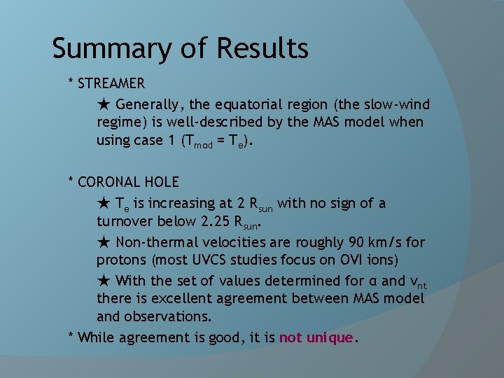
Summary of Results * STREAMER ★ Generally, the equatorial region (the slow-wind regime) is well-described by the MAS model when using case 1 (Tmod = Te). * CORONAL HOLE ★ Te is increasing at 2 Rsun with no sign of a turnover below 2. 25 Rsun. ★ Non-thermal velocities are roughly 90 km/s for protons (most UVCS studies focus on OVI ions) ★ With the set of values determined for α and vnt there is excellent agreement between MAS model and observations. * While agreement is good, it is not unique.

Future Work * Examine the MAS model and other MHD models for other periods in the solar cycle * Incorporate the data from O VI to add further constraints to the model parameters * Study an active region in the corona to see how shaped empirical heating function compares to observations Recommendations * MAS model should incorporate separate Te and Tp parameters (two-fluid physics) in order to be more physically accurate, or provide a better definition of which single temperature is calculated.

References Akinari, N. (2007). Broadening of resonantly scattered ultraviolet emission lines by coronal hole outflows. Ap. J, 660: 1660 -1673. Cranmer et al. (1999). An empirical model of a polar coronal hole at solar minimum. Ap. J, 511: 481. Jacques, S. A. (1977). Momentum and energy transport by waves in the solar atmosphere and solar wind. Ap. J, 215: 942 -951. Kohl et al. (1995). The Ultraviolet Coronagraph Spectrometer for the Solar and Heliospheric Observatory. Solar Physics, 162(1 -2): 313 -356. Landi, E. and Cranmer, S. R. (2009). Ion temperatures in the low solar corona: Polar coronal holes at solar minimum. Ap. J, 691: 794 -805. Lionello, R. , J. A. Linker, and Z. Mikić (2009). Multispectral emission of the Sun during the first whole Sun month: Magnetohydrodynamics simulations. Ap. J, 690: 902 -912. Ong et al. (1997). Self-consistent and time-dependent solar wind models. Ap. J, 474: L 143 -L 145. Withbroe, G. L. , J. L. Kohl, and H. Weiser (1982). Probing the solar wind acceleration region using spectroscopic techniques. Space Science Reviews, 33: 17 -52. THANK YOU!

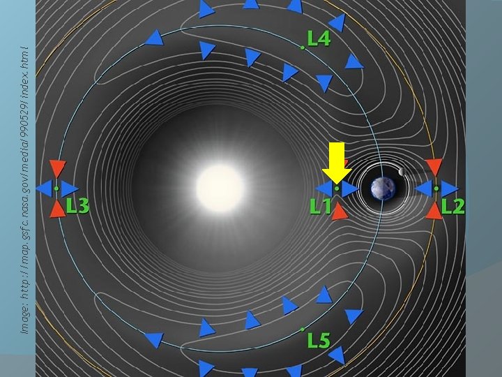
Image: http: //map. gsfc. nasa. gov/media/990529/index. html

UVCS Instrument Parameters * Ly-α channel Ruling frequency: 2400 l/mm Angle of incidence α: 12. 85° Angle of diffraction β: 3. 98° Main radius of curvature: 750 mm Minor radius of curvature: 729. 5 mm Reciprocal Dispersion: 5. 54 Å/mm (1 st order) Spectral Bandwidth of pixel: 0. 14 Å (1 st order) Spatial width of pixel: 0. 025 mm Image: http: //www. chrismadden. co. uk/moon/micro. html

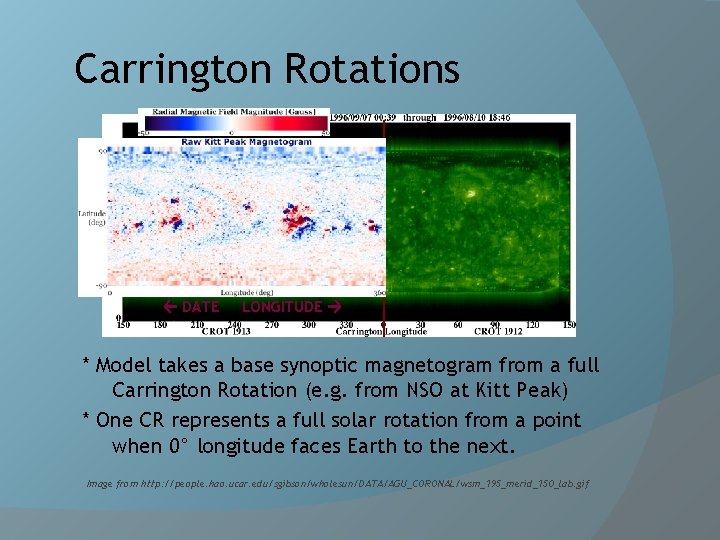
Carrington Rotations DATE LONGITUDE * Model takes a base synoptic magnetogram from a full Carrington Rotation (e. g. from NSO at Kitt Peak) * One CR represents a full solar rotation from a point when 0° longitude faces Earth to the next. Image from http: //people. hao. ucar. edu/sgibson/wholesun/DATA/AGU_CORONAL/wsm_195_merid_150_lab. gif

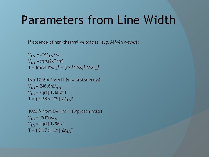
Parameters from Line Width If absence of non-thermal velocities (e. g. Alfvén waves): V 1/e = c*Δλ 1/e/λ 0 V 1/e = sqrt(2 k. T/m) T = (m/2 k)*V 1/e 2 = (mc 2/2 kλ 02)*Δλ 1/e 2 Lyα 1216 Å from H (m = proton mass) V 1/e = 246. 6*Δλ 1/e V 1/e = sqrt( T/60. 5 ) T = ( 3. 68 x 106 ) Δλ 1/e 2 1032 Å from OVI (m = 16*proton mass) V 1/e = 291*Δλ 1/e V 1/e = sqrt( T/965 ) T = ( 81. 7 x 106 ) Δλ 1/e 2

MAS Model {n, v, T, B} CORPRO Goal is to search for consistency between the MAS model and the UVCS Data by using Forward Modeling. UVCS Data { I(rows, col) } DAS v 40 “Modeled” { Itot, Δλ 1/e } “Observed” { Itot, Δλ 1/e } Data Map { I(λ) }