Empirical Model Empirical Models The empirical model represents

Empirical Model

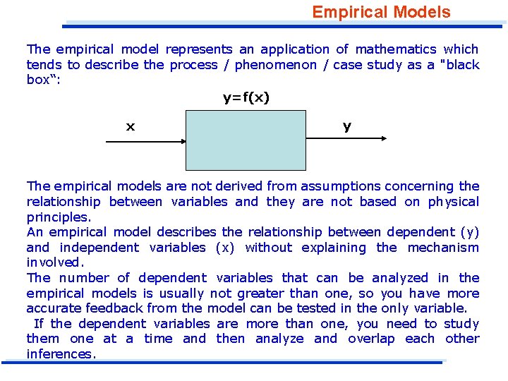
Empirical Models The empirical model represents an application of mathematics which tends to describe the process / phenomenon / case study as a "black box“: y=f(x) x y The empirical models are not derived from assumptions concerning the relationship between variables and they are not based on physical principles. An empirical model describes the relationship between dependent (y) and independent variables (x) without explaining the mechanism involved. The number of dependent variables that can be analyzed in the empirical models is usually not greater than one, so you have more accurate feedback from the model can be tested in the only variable. If the dependent variables are more than one, you need to study them one at a time and then analyze and overlap each other inferences.

Empirical Models The empirical model consists mainly in the formulation of a mathematical law that joins together the available experimental data, observations, etc. . in order to give answers relevant to the process / phenomenon / mechanism examined. An empirical model is entirely based on experimental data, observations, etc. . (Data Rich and Theory Poor) Each equation in the model includes one or more coefficients or parameters that are presumed constant. With the help of the experimental data, we can determine the form of the model, and subsequently (or simultaneously) estimate the value of some or all of the parameters in the model. Example: correlation that provides the specific heat at constant pressure, cp, as a function of temperature T: cp = a + b T where a and b are two constants that represent the parameters of the empirical model Note: this model provides an empirical model which employ 1 dependent variable and 1 independent variable A second example with more than 1 independent variable can be the algorithm of a multiple regression

Empirical Models Once the data is collected, you need to decide on the techniques you want to use in order to find an appropriate model. Depending on the type and quantity of data, and the characteristics of the problem, you can choose between two different approaches: 1. Interpolation: finding a function that contains all the data points. 2. Regression (Smoothing) or Model fitting: finding a function that is as close as possible to containing all the data points. Such function is also called a regression curve. Sometimes you would need to combine these methods since the interpolation curve might be too complex and the best fit model not to be sufficiently accurate

Empirical Models: Interpolation Assuming accurate data, we try to construct the curve that passes through the points representing the data "Interpolation guarantees the fitted curve will pass through each and every data point. “ Historically, the most famous and used interpolating functions are polynomials NOTE: the points awarded may NOT have the same abscissa, but ordinate different! SPLINE The interpolation by spline provides a different approach to the problem of interpolation. The spline are piecewise polynomial functions interpolating the function by keeping fixed the degree of the interpolating polynomial, but by dividing the entire interval of interpolation into n smaller sub-intervals and considering a different polynomial for each of these subintervals (same degree but different coefficients). In particular, the most considered are the cubic spline that are third degree.

Empirical Models: REGRESSION (SMOOTHING) It assumes the data with errors and tries to construct a curve which deviates slightly from the data, so as not to lose information contained in them "Regression simply ensures that the" merit function ", which is an arbitrary function that measures the disagreement between the data and the model, is minimized. "

Empirical Models: REGRESSION (SMOOTHING) Selection of the form of an empirical model requires judgment as well as some skill in organizing how response patterns match possible function. Optimization method can help in the selection of the model structure as well as in the estimation of the unknown coefficients. If you can specify a quantitative criterion which defines what is “best” in representing the data, then the model representation can be improved by adjustment of the form of the model to improve the value of he criterion. The best model, presumably, exhibits the least error between actual data and the predicted response in some sense.

The development of empirical models is divided into several phases: üPostulate of empirical model üMake an experimental plan and get data üAdaptation" of the model üEstimation of parameters üEvaluation of results In most cases, the development of empirical model goes through a cyclical process. Note: The construction work of the empirical model can be further improved using the techniques made available by the "Experimental Design".

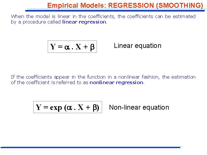
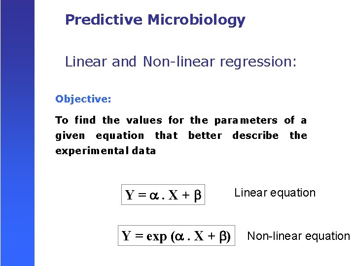
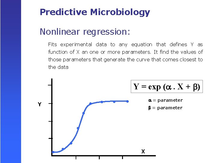
Empirical Models: REGRESSION (SMOOTHING) When the model is linear in the coefficients, the coefficients can be estimated by a procedure called linear regression. Y=. X+ Linear equation If the coefficients appear in the function in a nonlinear fashion, the estimation of the coefficient is referred to as nonlinear regression. Y = exp ( . X + ) Non-linear equation

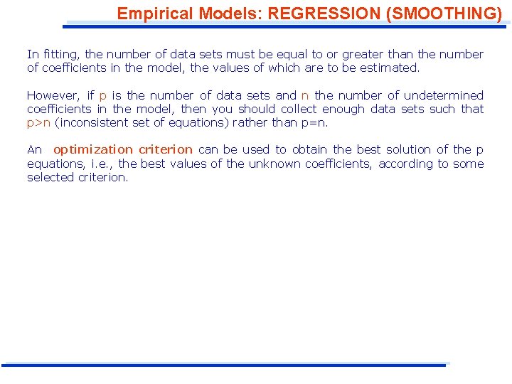
Empirical Models: REGRESSION (SMOOTHING) In fitting, the number of data sets must be equal to or greater than the number of coefficients in the model, the values of which are to be estimated. However, if p is the number of data sets and n the number of undetermined coefficients in the model, then you should collect enough data sets such that p>n (inconsistent set of equations) rather than p=n. An optimization criterion can be used to obtain the best solution of the p equations, i. e. , the best values of the unknown coefficients, according to some selected criterion.

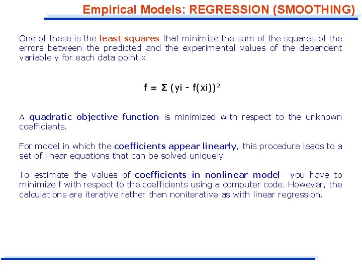
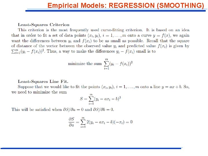
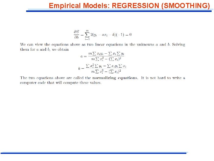
Empirical Models: REGRESSION (SMOOTHING) One of these is the least squares that minimize the sum of the squares of the errors between the predicted and the experimental values of the dependent variable y for each data point x. f = Σ (yi - f(xi))2 A quadratic objective function is minimized with respect to the unknown coefficients. For model in which the coefficients appear linearly, this procedure leads to a set of linear equations that can be solved uniquely. To estimate the values of coefficients in nonlinear model you have to minimize f with respect to the coefficients using a computer code. However, the calculations are iterative rather than noniterative as with linear regression.

Empirical Models: REGRESSION (SMOOTHING)

Empirical Models: REGRESSION (SMOOTHING)

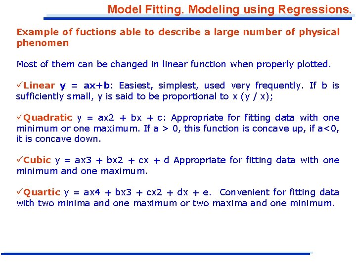
Model Fitting. Modeling using Regressions. Example of fuctions able to describe a large number of physical phenomen Most of them can be changed in linear function when properly plotted. üLinear y = ax+b: Easiest, simplest, used very frequently. If b is sufficiently small, y is said to be proportional to x (y / x); üQuadratic y = ax 2 + bx + c: Appropriate for fitting data with one minimum or one maximum. If a > 0, this function is concave up, if a<0, it is concave down. üCubic y = ax 3 + bx 2 + cx + d Appropriate for fitting data with one minimum and one maximum. üQuartic y = ax 4 + bx 3 + cx 2 + dx + e. Convenient for fitting data with two minima and one maximum or two maxima and one minimum.

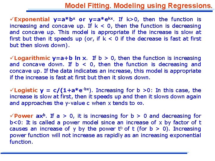
Model Fitting. Modeling using Regressions. üExponential y=a*bx or y=a*ekx. If k>0, then the function is increasing and concave up. If k < 0, then the function is decreasing and concave up. This model is appropriate if the increase is slow at first but then it speeds up (or, if k < 0 if the decrease is fast at first but then slows down). üLogarithmic y=a+b ln x. If b > 0, then the function is increasing and concave down. If b < 0, then the function is decreasing and concave up. If the data indicates an increase, this model is appropriate if the increase is fast at first but then it slows down. üLogistic y = c/(1+a*e-bx). Increasing for b >0: In this case, the increase is slow at first, then it speeds up and then it slows down again and approaches the y-value c when x tends to ∞. üPower axb. If a > 0, it is increasing for b > 0 and decreasing for b<0: It is called a power model since an increase of x by factor of t causes an increase of y by the power tb of t (for b > 0). Increasing power function will not increase as rapidly as an increasing exponential function.

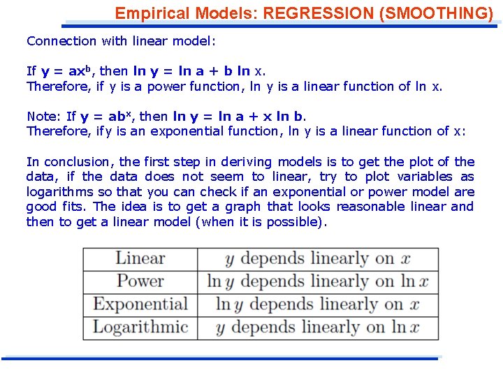
Empirical Models: REGRESSION (SMOOTHING) Connection with linear model: If y = axb, then ln y = ln a + b ln x. Therefore, if y is a power function, ln y is a linear function of ln x. Note: If y = abx, then ln y = ln a + x ln b. Therefore, ify is an exponential function, ln y is a linear function of x: In conclusion, the first step in deriving models is to get the plot of the data, if the data does not seem to linear, try to plot variables as logarithms so that you can check if an exponential or power model are good fits. The idea is to get a graph that looks reasonable linear and then to get a linear model (when it is possible).

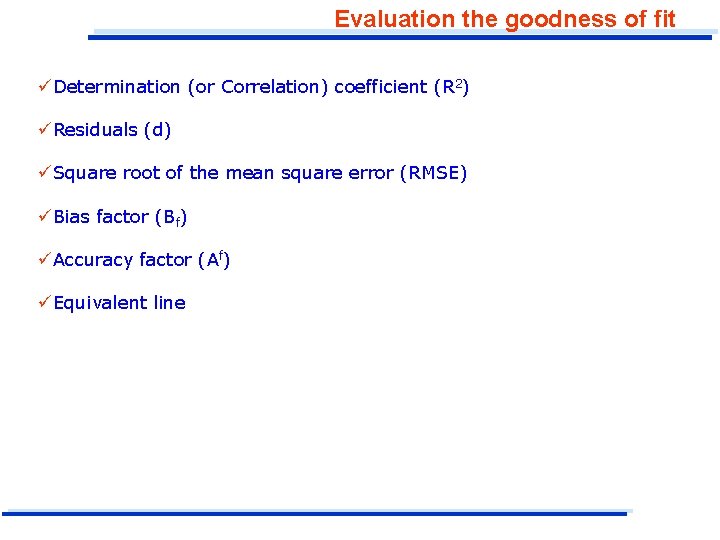
Evaluation the goodness of fit üDetermination (or Correlation) coefficient (R 2) üResiduals (d) üSquare root of the mean square error (RMSE) üBias factor (Bf) üAccuracy factor (Af) üEquivalent line

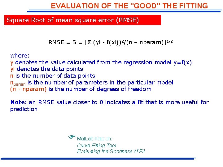
EVALUATION OF THE "GOOD" THE FITTING Square Root of mean square error (RMSE) RMSE = S = [Σ (yi - f(xi))2/(n – nparam)]1/2 where: y denotes the value calculated from the regression model y=f(x) yi denotes the data points n is the number of data points nparam is the number of parameters in the particular model (n - nparam) is the number of degrees of freedom Note: an RMSE value closer to 0 indicates a fit that is more useful for prediction Mat. Lab help on: Curve Fitting Tool Evaluating the Goodness of Fit

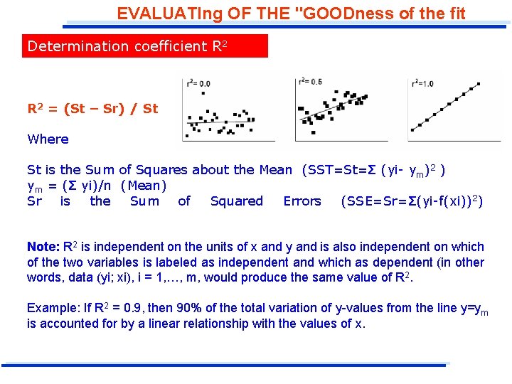
EVALUATIng OF THE "GOODness of the fit Determination coefficient R 2 = (St – Sr) / St Where St is the Sum of Squares about the Mean (SST=St=Σ (yi- ym)2 ) ym = (Σ yi)/n (Mean) Sr is the Sum of Squared Errors (SSE=Sr=Σ(yi-f(xi))2) Note: R 2 is independent on the units of x and y and is also independent on which of the two variables is labeled as independent and which as dependent (in other words, data (yi; xi), i = 1, …, m, would produce the same value of R 2. Example: If R 2 = 0. 9, then 90% of the total variation of y-values from the line y=ym is accounted for by a linear relationship with the values of x.

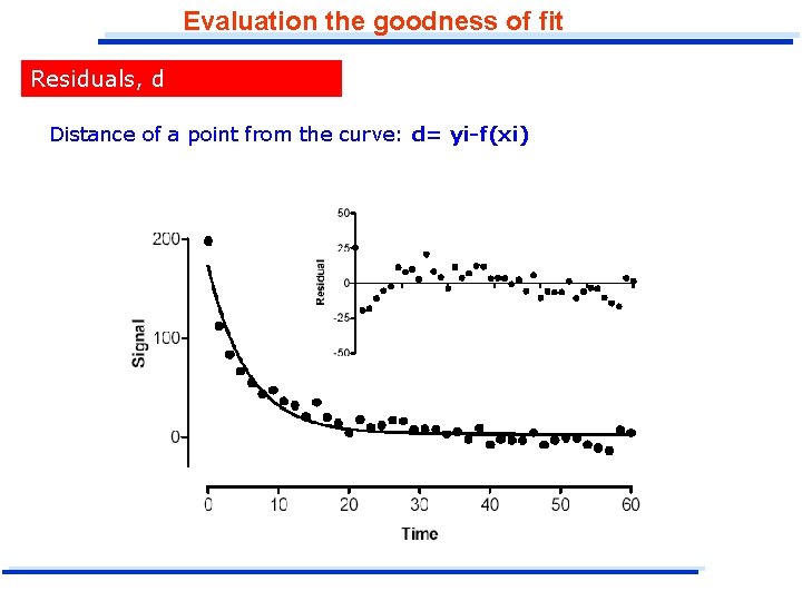
Evaluation the goodness of fit Residuals, d Distance of a point from the curve: d= yi-f(xi)

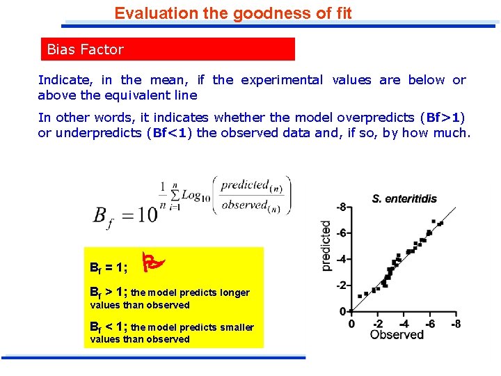
Evaluation the goodness of fit Bias Factor Indicate, in the mean, if the experimental values are below or above the equivalent line In other words, it indicates whether the model overpredicts (Bf>1) or underpredicts (Bf<1) the observed data and, if so, by how much. Bf = 1; Bf > 1; the model predicts longer values than observed Bf < 1; the model predicts smaller values than observed

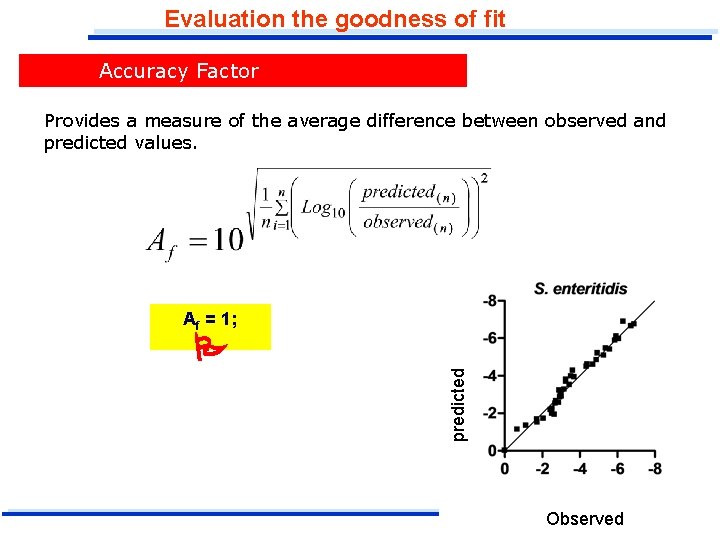
Evaluation the goodness of fit Accuracy Factor Provides a measure of the average difference between observed and predicted values. Af = 1; predicted Observed

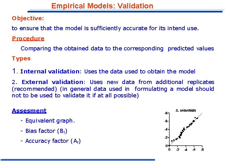
Empirical Models: Validation Objective: to ensure that the model is sufficiently accurate for its intend use. Procedure Comparing the obtained data to the corresponding predicted values Types 1. Internal validation: Uses the data used to obtain the model 2. External validation: Uses new data from additional replicates (recommended) (in general data used in formulating a model should not to be used to validate it if at all possible) Assesment - Equivalent graph. - Bias factor (Bf) - Accuracy factor (Af)

Predictive Microbiology Linear and Non-linear regression: Objective: To find the values for the parameters of a given equation that better describe the experimental data Y=. X+ Y = exp ( . X + ) Linear equation Non-linear equation

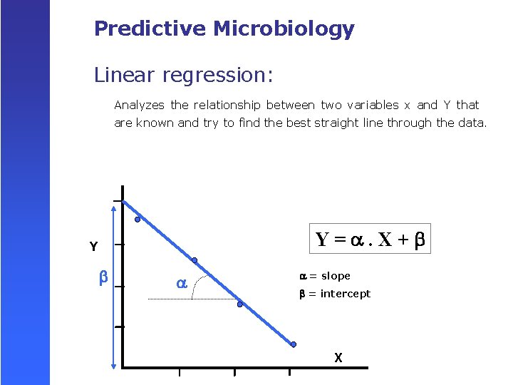
Predictive Microbiology Linear regression: Analyzes the relationship between two variables x and Y that are known and try to find the best straight line through the data. Y=. X+ Y = slope = intercept X

Predictive Microbiology Nonlinear regression: Fits experimental data to any equation that defines Y as function of X an one or more parameters. It find the values of those parameters that generate the curve that comes closest to the data Y = exp ( . X + ) = parameter Y = parameter X

Predictive Microbiology Inactivation models number of survivors 60ºC Nt = No e-kt Treatment time

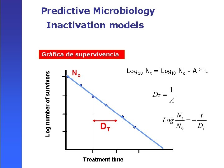
Predictive Microbiology Inactivation models Log number of survivors Gráfica de supervivencia Log 10 Nt = Log 10 No - A * t No DT Treatment time

Predictive Microbiology Inactivation models Log Number of survivors Survival line 50ºC D 71ºC 70ºC D 50ºC D 60ºC Treatment time

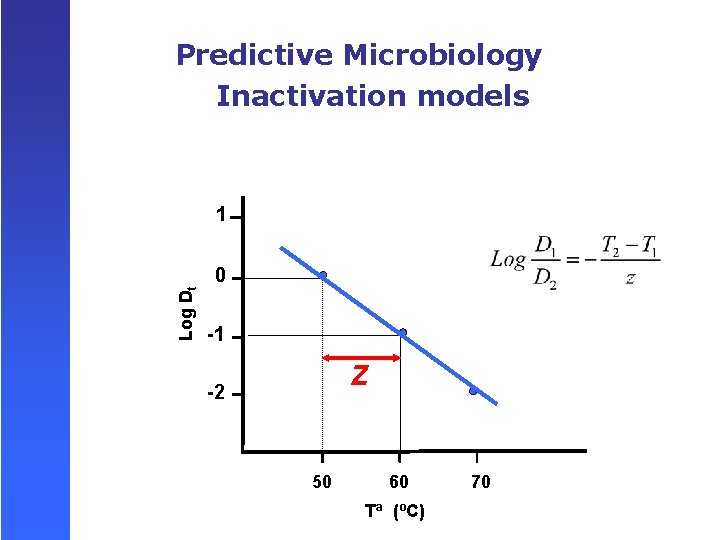
Predictive Microbiology Inactivation models Log Dt 1 0 -1 Z -2 50 60 Tª (ºC) 70

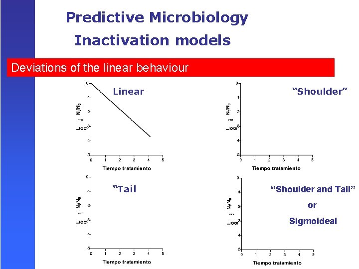
Predictive Microbiology Inactivation models Deviations of the linear behaviour Linear “Tail “Shoulder” “Shoulder and Tail” or Sigmoideal

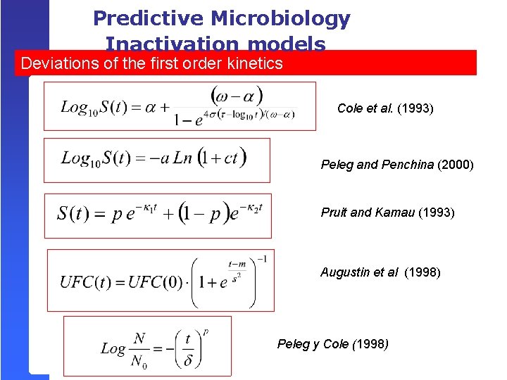
Predictive Microbiology Inactivation models Deviations of the first order kinetics Cole et al. (1993) Peleg and Penchina (2000) Pruit and Kamau (1993) Augustin et al (1998) Peleg y Cole (1998)

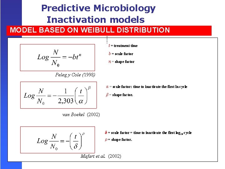
Predictive Microbiology Inactivation models MODEL BASED ON WEIBULL DISTRIBUTION t = treatment time b = scale factor n = shape factor Peleg y Cole (1998) α = scale factor: time to inactivate the first ln cycle β = shape factor. van Boekel (2002) δ = scale factor = time to inactivate the first log 10 cycle p = shape factor. Mafart et al. (2002)

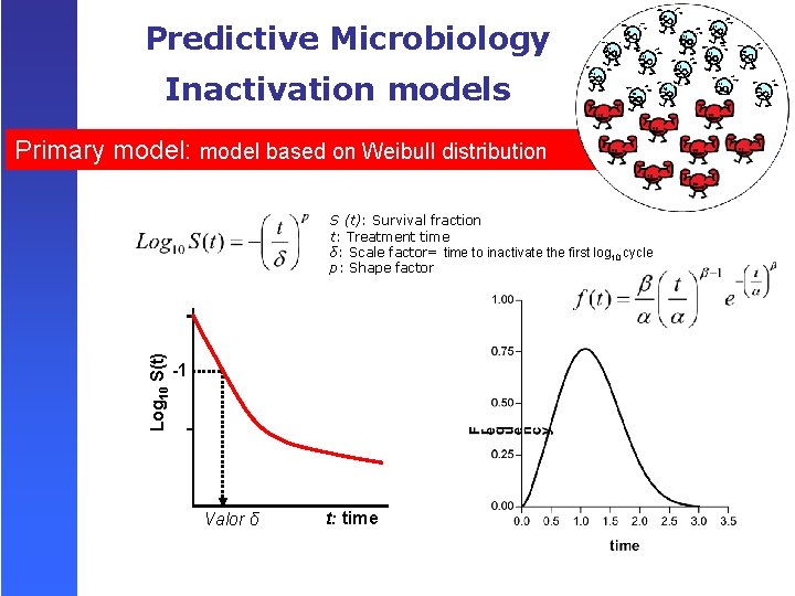
Predictive Microbiology Inactivation models Primary model: model based on Weibull distribution Log 10 S(t) S (t): Survival fraction t: Treatment time δ: Scale factor= time to inactivate the first log 10 cycle p: Shape factor -1 Valor δ t: time

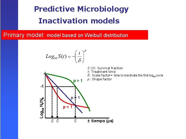
Predictive Microbiology Inactivation models Primary model: model based on Weibull distribution p>1 S (t): Survival fraction t: Treatment time δ: Scale factor= time to inactivate the first log 10 cycle p: Shape factor -1 Log 10 Nt/N 0 p=1 p<1 δ δ δ t: tiempo (µs)