Empirical Methods for Microeconomic Applications University of Lugano


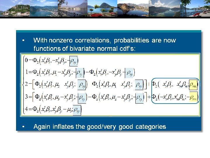
: • • • Functional form strategy")


 • • •")


: • • More classes")


 Model")


 = Pr(true) * Pr(y | true)")


 Log")


![Simulating Conditional Means for Individual Parameters Posterior estimates of E[parameters(i) | Data(i)]](https://slidetodoc.com/presentation_image_h/2285a9299dc53cf86edc1db30eacabb3/image-63.jpg "Simulating Conditional Means for Individual Parameters Posterior estimates of E[parameters(i) | Data(i)]")


- Slides: 68
Empirical Methods for Microeconomic Applications University of Lugano, Switzerland May 27 -31, 2013 William Greene Department of Economics Stern School of Business
2 B. Heterogeneity: Latent Class and Mixed Models
Agenda for 2 B • • • Latent Class and Finite Mixtures Random Parameters Multilevel Models
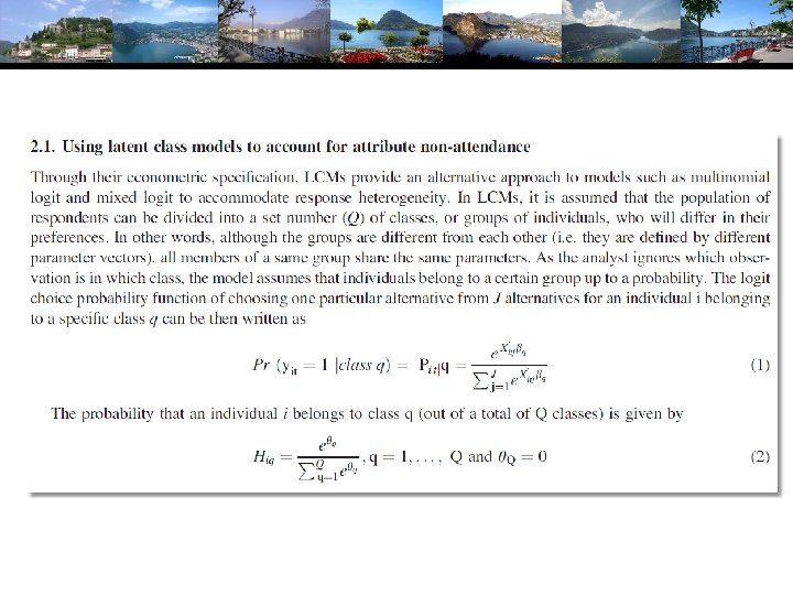
Latent Classes • • A population contains a mixture of individuals of different types (classes) Common form of the data generating mechanism within the classes Observed outcome y is governed by the common process F(y|x, j ) Classes are distinguished by the parameters, j.
How Finite Mixture Models Work Density? Note significant mass below zero. Not a gamma or lognormal or any other familiar density.
Find the ‘Best’ Fitting Mixture of Two Normal Densities
Mixing probabilities. 715 and. 285
Approximation Actual Distribution
A Practical Distinction • Finite Mixture (Discrete Mixture): • • • Functional form strategy Component densities have no meaning Mixing probabilities have no meaning There is no question of “class membership” The number of classes is uninteresting – enough to get a good fit Latent Class: • • • Mixture of subpopulations Component densities are believed to be definable “groups” (Low Users and High Users in Bago d’Uva and Jones application) The classification problem is interesting – who is in which class? Posterior probabilities, P(class|y, x) have meaning Question of the number of classes has content in the context of the analysis
The Latent Class Model
Log Likelihood for an LC Model
Estimating Which Class
‘Estimating’ βi
How Many Classes?
The Extended Latent Class Model
Unfortunately, this argument is incorrect.
Zero Inflation?
Zero Inflation – ZIP Models • Two regimes: (Recreation site visits) • • • Unconditional: • • • Zero (with probability 1). (Never visit site) Poisson with Pr(0) = exp[- ’xi]. (Number of visits, including zero visits this season. ) Pr[0] = P(regime 0) + P(regime 1)*Pr[0|regime 1] Pr[j | j >0] = P(regime 1)*Pr[j|regime 1] This is a “latent class model”
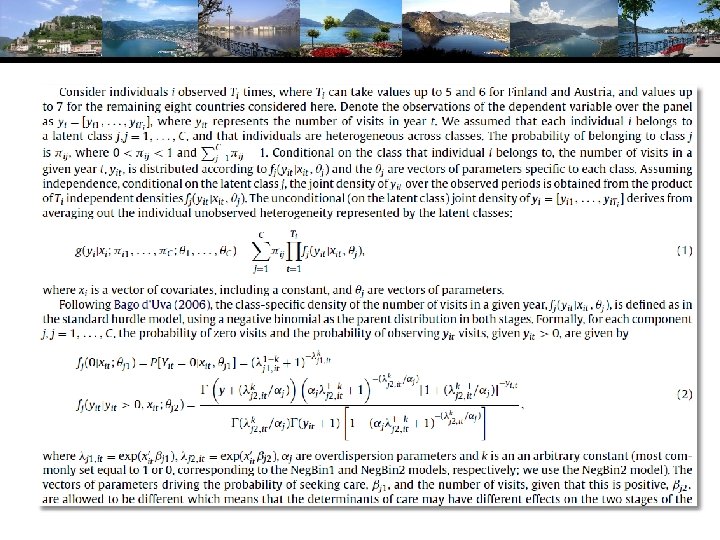
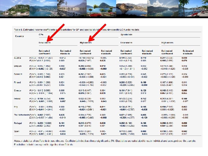
A Latent Class Hurdle NB 2 Model • • Analysis of ECHP panel data (1994 -2001) Two class Latent Class Model • • Typical in health economics applications Hurdle model for physician visits • • Poisson hurdle for participation and negative binomial intensity given participation Contrast to a negative binomial model
LC Poisson Regression for Doctor Visits
Heckman and Singer’s RE Model • • Random Effects Model Random Constants with Discrete Distribution
3 Class Heckman-Singer Form
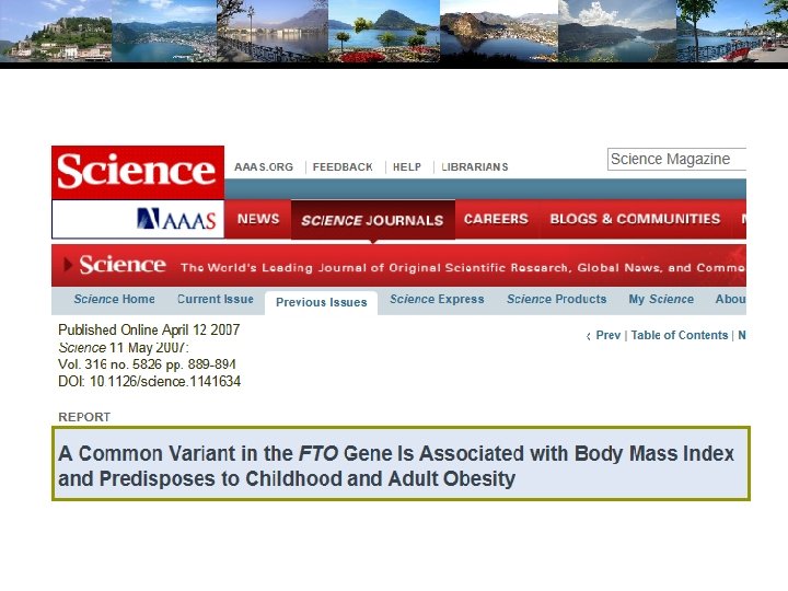
Modeling Obesity with a Latent Class Model Mark Harris Department of Economics, Curtin University Bruce Hollingsworth Department of Economics, Lancaster University William Greene Stern School of Business, New York University Pushkar Maitra Department of Economics, Monash University
Two Latent Classes: Approximately Half of European Individuals
An Ordered Probit Approach A Latent Regression Model for “True BMI” BMI* = ′x + , ~ N[0, σ2], σ2 = 1 “True BMI” = a proxy for weight is unobserved Observation Mechanism for Weight Type WT = 0 if 1 if 2 if BMI* < 0 0 < BMI* < < BMI* Normal Overweight Obese
Latent Class Modeling • Several ‘types’ or ‘classes. Obesity be due to genetic reasons (the FTO gene) or lifestyle factors • Distinct sets of individuals may have differing reactions to various policy tools and/or characteristics • The observer does not know from the data which class an individual is in. • Suggests a latent class approach for health outcomes (Deb and Trivedi, 2002, and Bago d’Uva, 2005)
Latent Class Application • Two class model (considering FTO gene): • • More classes make class interpretations much more difficult Parametric models proliferate parameters Endogenous class membership: Two classes allow us to correlate the equations driving class membership and observed weight outcomes via unobservables. Theory for more than two classes not yet developed.
Endogeneity of Class Membership
Outcome Probabilities • • • Class 0 dominated by normal and overweight probabilities ‘normal weight’ class Class 1 dominated by probabilities at top end of the scale ‘non-normal weight’ Unobservables for weight class membership, negatively correlated with those determining weight levels:
Classification (Latent Probit) Model
Inflated Responses in Self-Assessed Health Mark Harris Department of Economics, Curtin University Bruce Hollingsworth Department of Economics, Lancaster University William Greene Stern School of Business, New York University
SAH vs. Objective Health Measures Favorable SAH categories seem artificially high. 60% of Australians are either overweight or obese (Dunstan et. al, 2001) 1 in 4 Australians has either diabetes or a condition of impaired glucose metabolism Over 50% of the population has elevated cholesterol Over 50% has at least 1 of the “deadly quartet” of health conditions (diabetes, obesity, high blood pressure, high cholestrol) Nearly 4 out of 5 Australians have 1 or more long term health conditions (National Health Survey, Australian Bureau of Statistics 2006) Australia ranked #1 in terms of obesity rates Similar results appear to appear for other countries
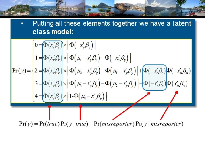
A Two Class Latent Class Model True Reporter Misreporter
• • Mis-reporters choose either good or very good The response is determined by a probit model Y=3 Y=2
Y=4 Y=3 Y=2 Y=1 Y=0
Observed Mixture of Two Classes
Pr(true, y) = Pr(true) * Pr(y | true)
General Result 0. 4 0. 35 0. 3 0. 25 Sample Predicted Mis-Reporting 0. 2 0. 15 0. 1 0. 05 0 Poor Fair Good Very Good Excellent
RANDOM PARAMETER MODELS
A Recast Random Effects Model
A Computable Log Likelihood
Simulation
Random Effects Model: Simulation -----------------------------------Random Coefficients Probit Model Dependent variable DOCTOR (Quadrature Based) Log likelihood function -16296. 68110 (-16290. 72192) Restricted log likelihood -17701. 08500 Chi squared [ 1 d. f. ] 2808. 80780 Simulation based on 50 Halton draws ----+------------------------Variable| Coefficient Standard Error b/St. Er. P[|Z|>z] ----+------------------------|Nonrandom parameters AGE|. 02226***. 00081 27. 365. 0000 (. 02232) EDUC| -. 03285***. 00391 -8. 407. 0000 (-. 03307) HHNINC|. 00673. 05105. 132. 8952 (. 00660) |Means for random parameters Constant| -. 11873**. 05950 -1. 995. 0460 (-. 11819) |Scale parameters for dists. of random parameters Constant|. 90453***. 01128 80. 180. 0000 ----+------------------------------- Implied from these estimates is. 904542/(1+. 904532) =. 449998.
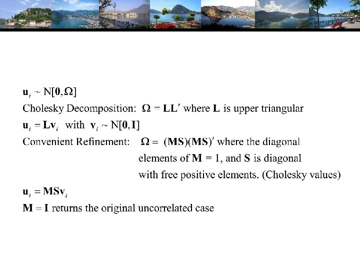
Recast the Entire Parameter Vector
S M
MSS M
Modeling Parameter Heterogeneity
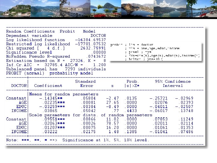
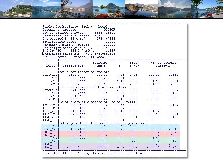
Hierarchical Probit Model Uit = 1 i + 2 i. Ageit + 3 i. Educit + 4 i. Incomeit + it. 1 i= 1+ 11 Femalei + 12 Marriedi + u 1 i 2 i= 2+ 21 Femalei + 22 Marriedi + u 2 i 3 i= 3+ 31 Femalei + 32 Marriedi + u 3 i 4 i= 4+ 41 Femalei + 42 Marriedi + u 4 i Yit = 1[Uit > 0] All random variables normally distributed.
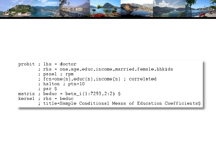
Simulating Conditional Means for Individual Parameters Posterior estimates of E[parameters(i) | Data(i)]
Probit
“Individual Coefficients”
Mixed Model Estimation Programs differ on the models fitted, the algorithms, the paradigm, and the extensions provided to the simplest RPM, i = +wi. • • Win. BUGS: • MCMC • User specifies the model – constructs the Gibbs Sampler/Metropolis Hastings MLWin: • Linear and some nonlinear – logit, Poisson, etc. • Uses MCMC for MLE (noninformative priors) SAS: Proc Mixed. • Classical • Uses primarily a kind of GLS/GMM (method of moments algorithm for loglinear models) Stata: Classical • Several loglinear models – GLAMM. Mixing done by quadrature. • Maximum simulated likelihood for multinomial choice (Arne Hole, user provided) LIMDEP/NLOGIT • Classical • Mixing done by Monte Carlo integration – maximum simulated likelihood • Numerous linear, nonlinear, loglinear models Ken Train’s Gauss Code • Monte Carlo integration • Mixed Logit (mixed multinomial logit) model only (but free!) Biogeme • Multinomial choice models • Many experimental models (developer’s hobby)