Empirical Bayes Gene Detection in Microarray Analysis Prepared

Empirical Bayes Gene Detection in Microarray Analysis Prepared for NZSA 2005 Conference Department of Statistics The University of Auckland Sarah Song: qson 003@stat. auckland. ac. nz 12/29/2021 1

Overview • • • Introduction Problem and Aim Methodology DLBCL data Evaluation Discussion 12/29/2021 2

Introduction (1) What is microarray analysis? • Thousands of genes in a single • • experiment Detect gene mutations or differential expression (the change of activities of genes) M Schena, D Shalon, RW Davis, PO Brown (1995) “Quantitative monitoring of gene-expression patterns with a complementary-DNA microarray”, Science, 270(5235): 467 -470 12/29/2021 3

Introduction (2) • • Application of Microarray § Survival analysis Example: Diffuse large B-cell lymphoma (Alizadeh et al. , 2000) § § § 12/29/2021 7399 gene expression profiles (microarray) 240 patients (160 patients in training data; 80 patients in test data) Censored survival times (138 failure, 102 censored) 4

Introduction (3) • Current work on DLBCL data (1) Hierarchical clustering (Alizadeh et al. , 2000) or Supervised learning (Shipp et al. , 2002): Identify subgroups of patients (2) Survival analysis (Bair&Tibshirani, 2003): Predict patients’ survival times • Our work on this data § 12/29/2021 Select a suitable model gene times 5

Problem and Aim Data structure • No. of variables (7399) >> No. of samples (240) Problem • • • Many statistical analyses are difficult to implement Overfitting AIC, BIC do not work properly Aim • • • A special selection method (overcome problems) A new threshold A best possible model 12/29/2021 6

Methodology (1) Nonparametric Empirical Bayes(EB) • • • Estimate the latent distribution (mixture model of chi-distribution) Bayes parameters are estimated based on the observed data Number of components is unbounded 12/29/2021 7

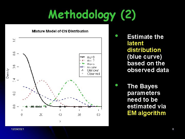
Methodology (2) 12/29/2021 • Estimate the latent distribution (blue curve) based on the observed data • The Bayes parameters need to be estimated via EM algorithm 8

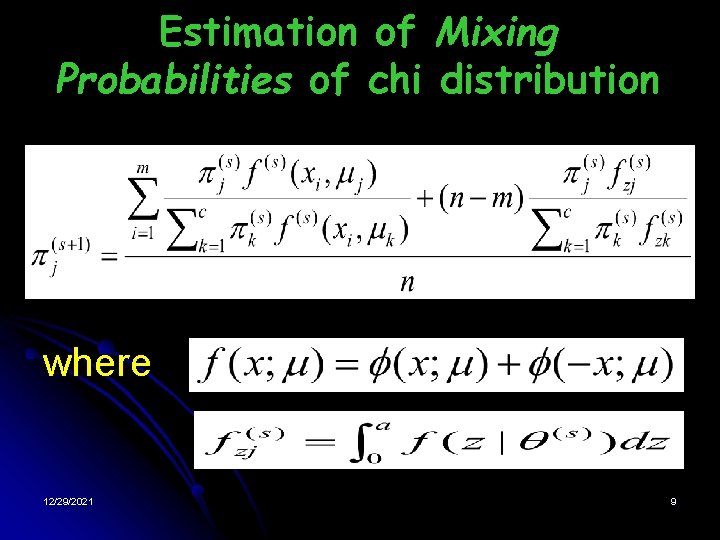
Estimation of Mixing Probabilities of chi distribution where 12/29/2021 9

Estimation of centers of the univariate components 12/29/2021 10

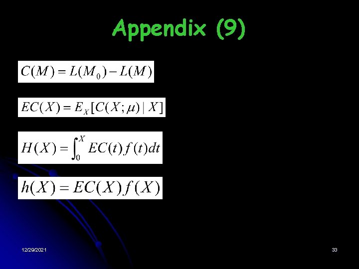
Methodology (3) • Projection Adjustment by Contribution Estimation (Wang, 2002) § PACE 2 procedure: The model has the largest cumulated expected contribution at the optimal point. Note: Maximizing the cumulated expected contribution is equivalent to maximizing the expected log-likelihood 12/29/2021 11

Example: DLBCL (1) Question: Are there any genes which, individually, are significantly related to survival times? Example: • Data: 7399 gene with 240 patient (160 patients in training data; 80 patients in test data) • • • Model: Cox proportional hazards model Imputation: 10 Nearest Neighbors method (Hastie & Tibshirani, 1999) Plan: Estimate latent distribution based on the observed data (loglikelihood) 12/29/2021 12

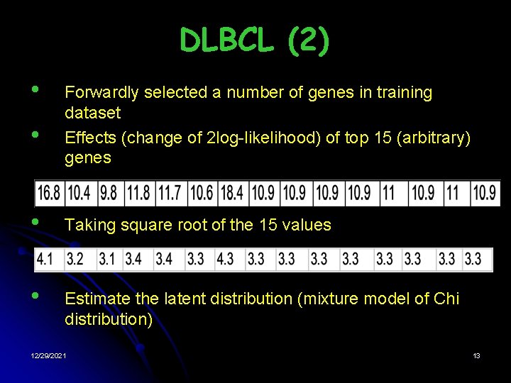
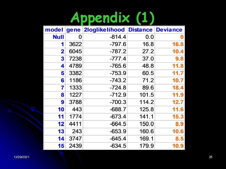
DLBCL (2) • • Forwardly selected a number of genes in training dataset Effects (change of 2 log-likelihood) of top 15 (arbitrary) genes • Taking square root of the 15 values • Estimate the latent distribution (mixture model of Chi distribution) 12/29/2021 13

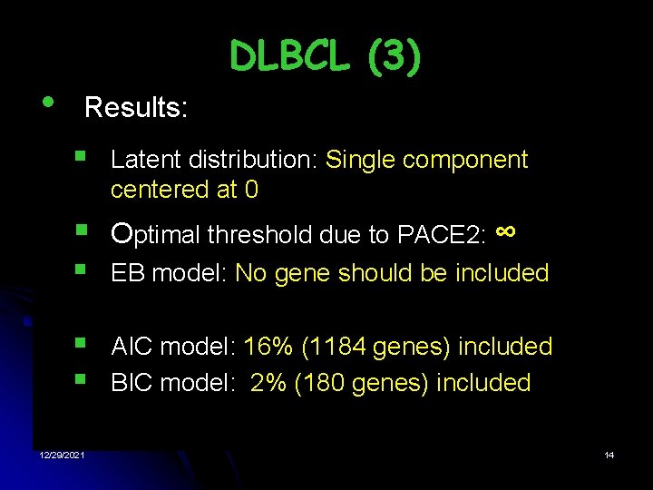
• DLBCL (3) Results: § Latent distribution: Single component centered at 0 § Optimal threshold due to PACE 2: ∞ § EB model: No gene should be included § § AIC model: 16% (1184 genes) included BIC model: 2% (180 genes) included 12/29/2021 14

Evaluation • Fitting the independent test data • Hypothesis testing • Fitting simulation dataset 12/29/2021 15

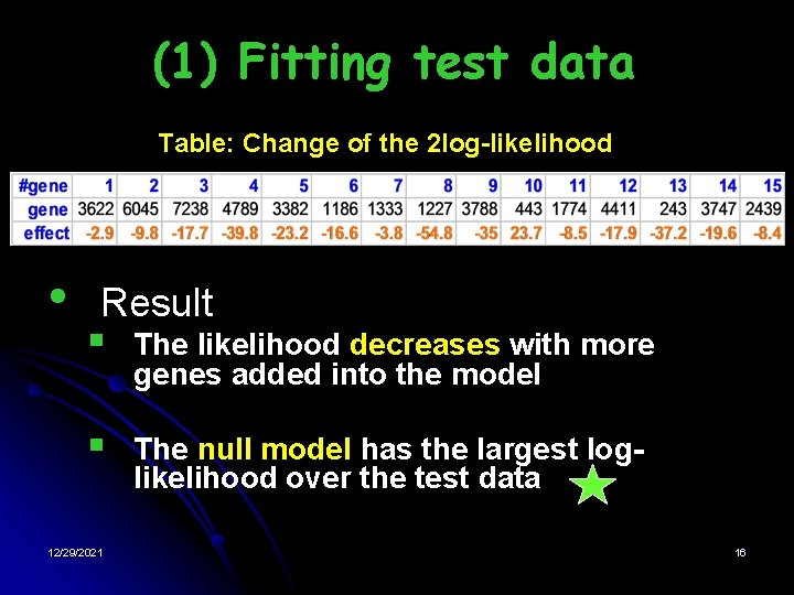
(1) Fitting test data Table: Change of the 2 log-likelihood • Result § The likelihood decreases with more genes added into the model § 12/29/2021 The null model has the largest loglikelihood over the test data 16

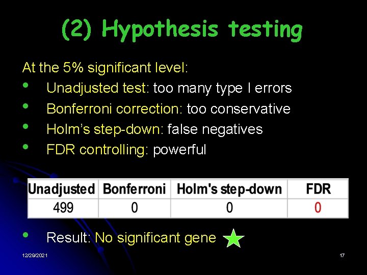
(2) Hypothesis testing At the 5% significant level: • Unadjusted test: too many type I errors • Bonferroni correction: too conservative • Holm’s step-down: false negatives • FDR controlling: powerful • Result: No significant gene 12/29/2021 17

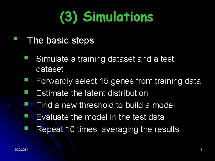
(3) Simulations • The basic steps § § § 12/29/2021 Simulate a training dataset and a test dataset Forwardly select 15 genes from training data Estimate the latent distribution Find a new threshold to build a model Evaluate the model in the test data Repeat 10 times, averaging the results 18

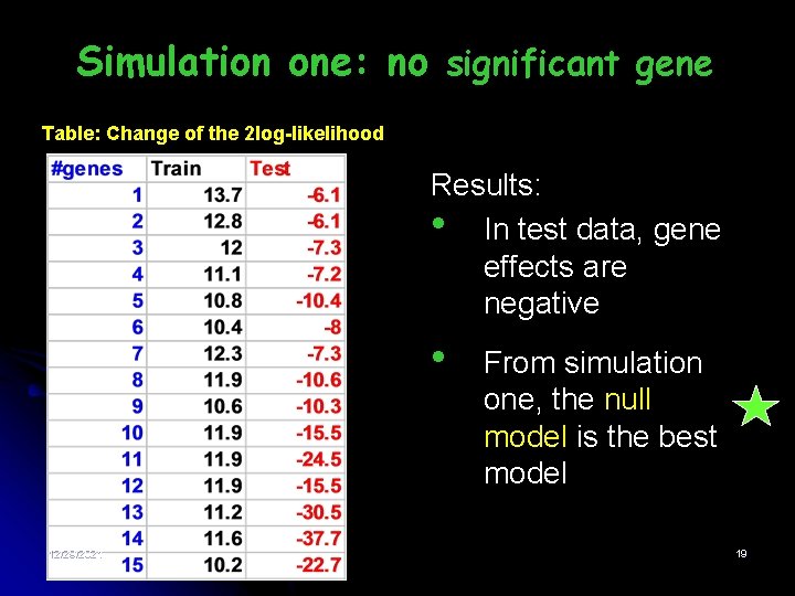
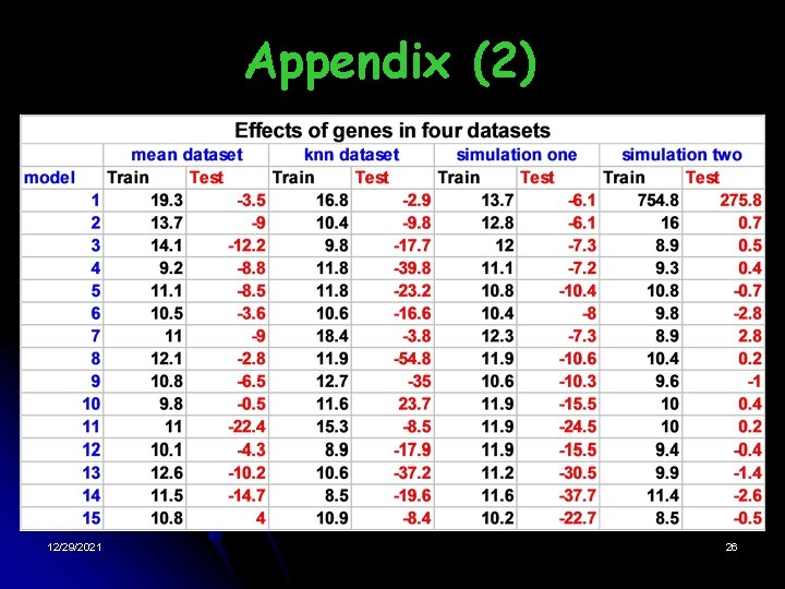
Simulation one: no significant gene Table: Change of the 2 log-likelihood Results: • In test data, gene effects are negative • 12/29/2021 From simulation one, the null model is the best model 19

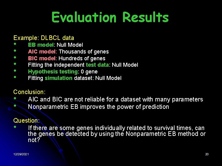
Evaluation Results Example: DLBCL data • • • EB model: Null Model AIC model: Thousands of genes BIC model: Hundreds of genes Fitting the independent test data: Null Model Hypothesis testing: 0 gene Fitting simulation dataset: Null Model Conclusion: • AIC and BIC are not reliable for a dataset with many parameters • Nonparametric EB improves the power of prediction Question: • If there are some genes individually related to survival times, can the genes be detected by using the Nonparametric EB method or not? 12/29/2021 20

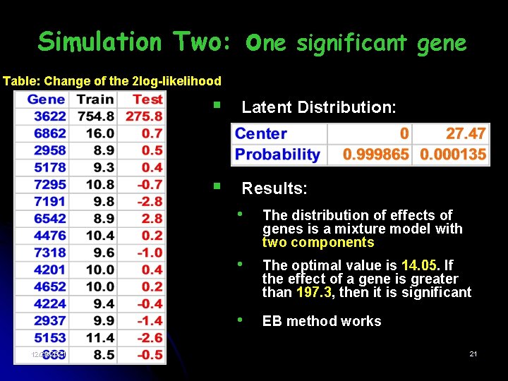
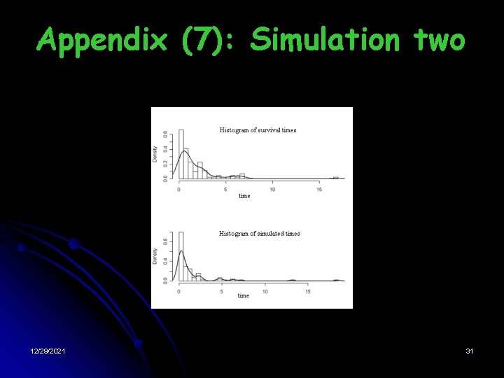
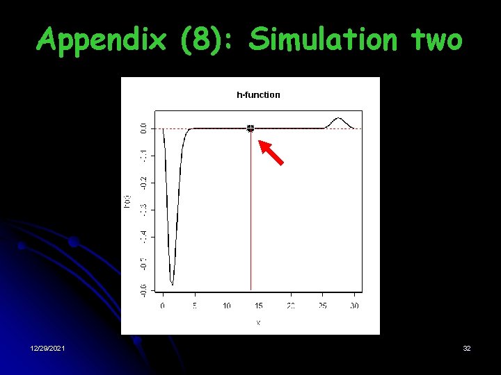
one Simulation Two: significant gene Table: Change of the 2 log-likelihood 12/29/2021 § Latent Distribution: § Results: • The distribution of effects of genes is a mixture model with two components • The optimal value is 14. 05. If the effect of a gene is greater than 197. 3, then it is significant • EB method works 21

Discussion • Conclusion § § § • Nonparametric EB method can help solve the overfitting problem AIC and BIC are not reliable for a dataset with many parameters Nonparametric EB method is a very useful tool for obtaining accurate models in the large-scaled datasets (e. g. , microarray data) Future work § § 12/29/2021 Apply Nonparametric EB on grouped genes Other threshold methods in microarray analysis • • Cross-validation Shrinkage methods 22

Acknowledgements • • Yong Wang (The University of Auckland) Mik Black (The University of Auckland) The Department of Statistics (The University of Auckland) New Zealand Statistical Association 12/29/2021 23

Thank you =) 12/29/2021 24

Appendix (1) 12/29/2021 25

Appendix (2) 12/29/2021 26

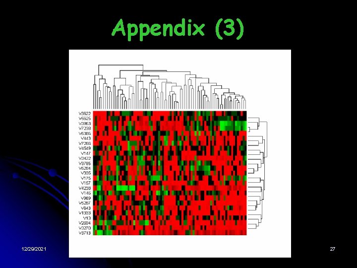
Appendix (3) 12/29/2021 27

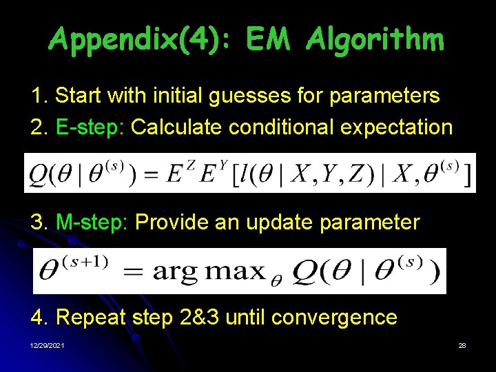
Appendix(4): EM Algorithm 1. Start with initial guesses for parameters 2. E-step: Calculate conditional expectation 3. M-step: Provide an update parameter 4. Repeat step 2&3 until convergence 12/29/2021 28

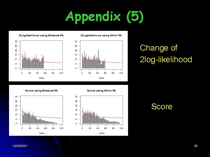
Appendix (5) • • • 12/29/2021 Change of 2 log-likelihood Score 29

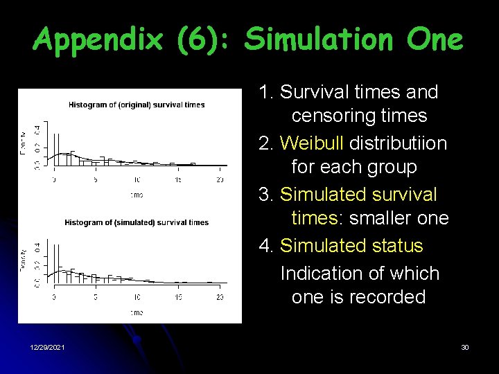
Appendix (6): Simulation One 1. Survival times and censoring times 2. Weibull distributiion for each group 3. Simulated survival times: smaller one 4. Simulated status Indication of which one is recorded 12/29/2021 30

Appendix (7): Simulation two 12/29/2021 31

Appendix (8): Simulation two 12/29/2021 32

Appendix (9) 12/29/2021 33