EM algorithm LING 572 Fei Xia 030206 Outline

EM algorithm LING 572 Fei Xia 03/02/06

Outline • The EM algorithm • EM for PM models • Three special cases – Inside-outside algorithm – Forward-backward algorithm – IBM models for MT

The EM algorithm

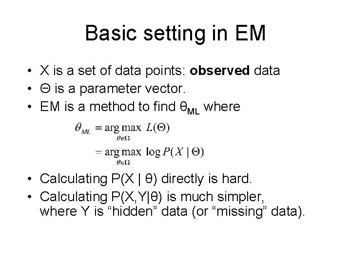
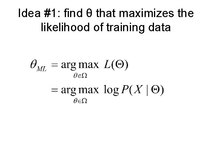
Basic setting in EM • X is a set of data points: observed data • Θ is a parameter vector. • EM is a method to find θML where • Calculating P(X | θ) directly is hard. • Calculating P(X, Y|θ) is much simpler, where Y is “hidden” data (or “missing” data).

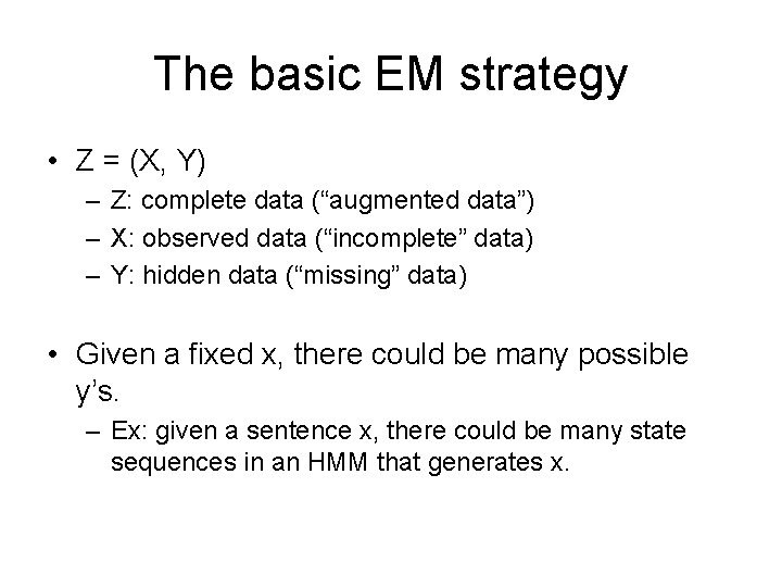
The basic EM strategy • Z = (X, Y) – Z: complete data (“augmented data”) – X: observed data (“incomplete” data) – Y: hidden data (“missing” data) • Given a fixed x, there could be many possible y’s. – Ex: given a sentence x, there could be many state sequences in an HMM that generates x.

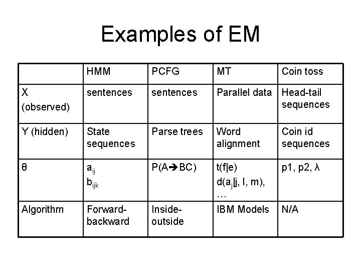
Examples of EM HMM PCFG MT Coin toss X (observed) sentences Parallel data Head-tail sequences Y (hidden) State sequences Parse trees Word alignment Coin id sequences θ aij bijk P(A BC) t(f|e) d(aj|j, l, m), … p 1, p 2, λ Algorithm Forwardbackward Insideoutside IBM Models N/A

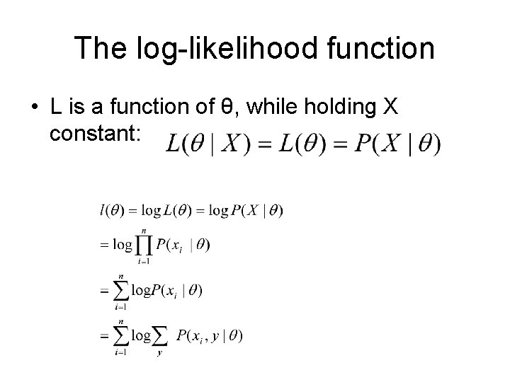
The log-likelihood function • L is a function of θ, while holding X constant:

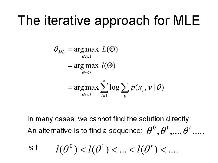
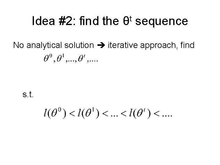
The iterative approach for MLE In many cases, we cannot find the solution directly. An alternative is to find a sequence: s. t.

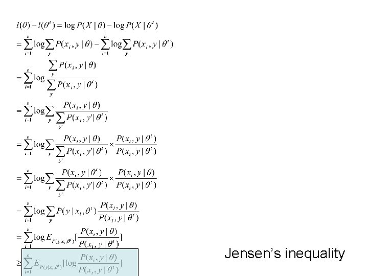
Jensen’s inequality

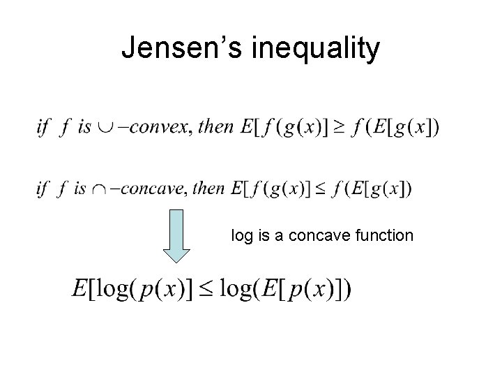
Jensen’s inequality log is a concave function

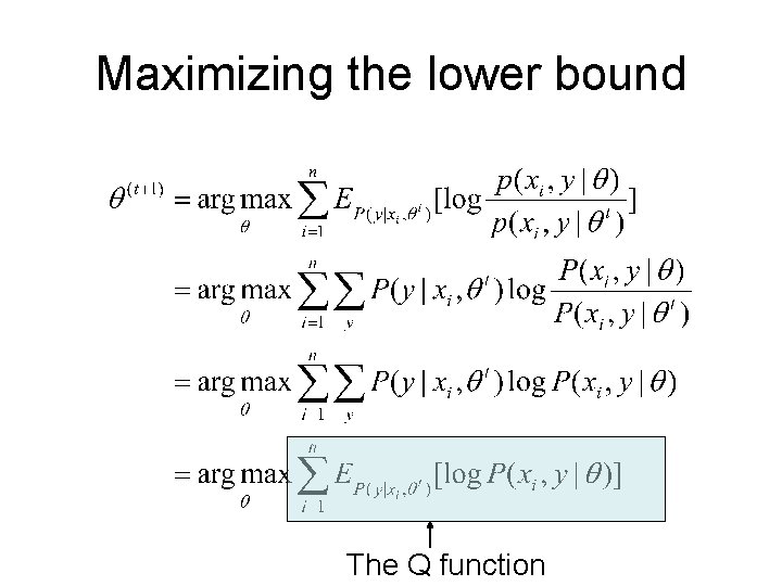
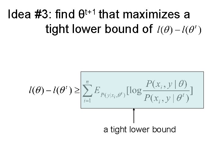
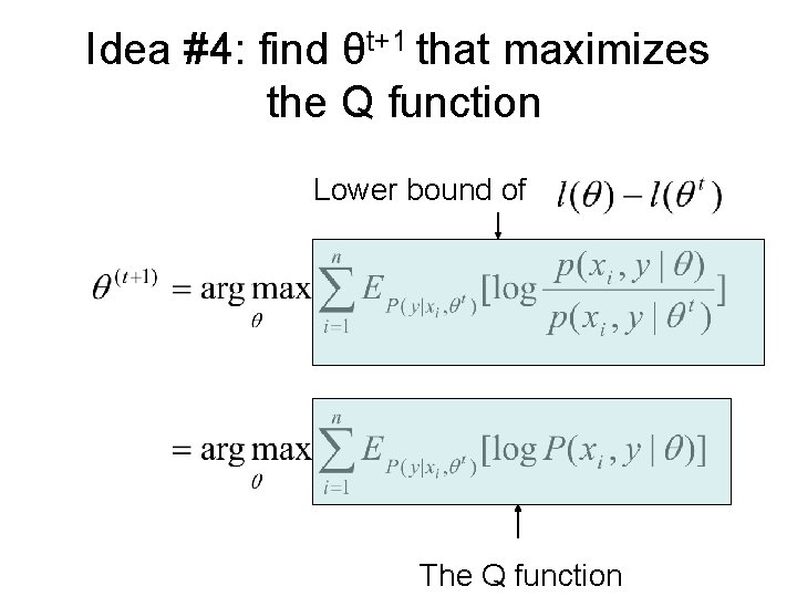
Maximizing the lower bound The Q function

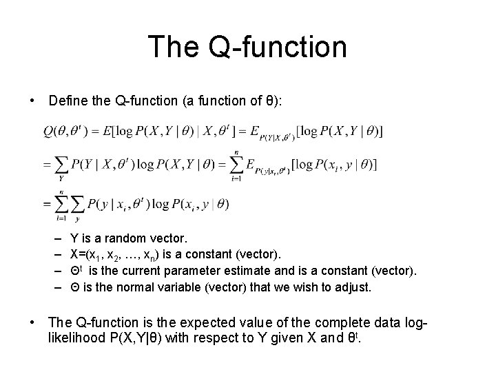
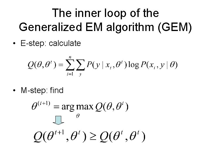
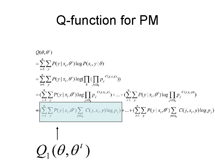
The Q-function • Define the Q-function (a function of θ): – – Y is a random vector. X=(x 1, x 2, …, xn) is a constant (vector). Θt is the current parameter estimate and is a constant (vector). Θ is the normal variable (vector) that we wish to adjust. • The Q-function is the expected value of the complete data loglikelihood P(X, Y|θ) with respect to Y given X and θt.

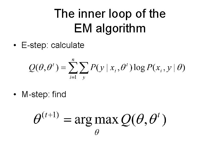
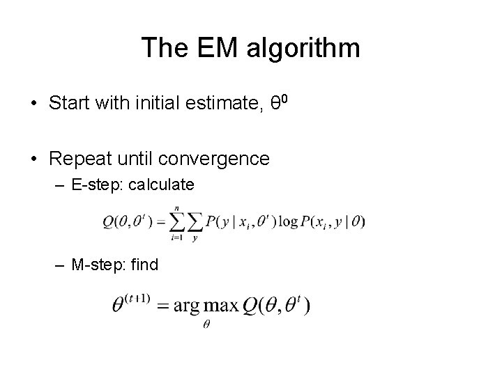
The inner loop of the EM algorithm • E-step: calculate • M-step: find

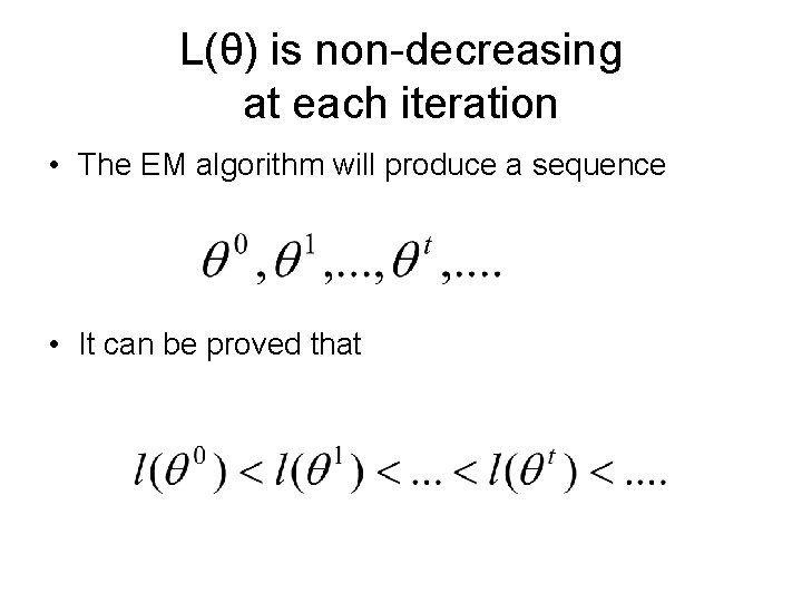
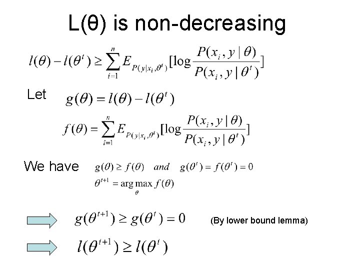
L(θ) is non-decreasing at each iteration • The EM algorithm will produce a sequence • It can be proved that

The inner loop of the Generalized EM algorithm (GEM) • E-step: calculate • M-step: find

Recap of the EM algorithm

Idea #1: find θ that maximizes the likelihood of training data

Idea #2: find the θt sequence No analytical solution iterative approach, find s. t.

Idea #3: find θt+1 that maximizes a tight lower bound of a tight lower bound

Idea #4: find θt+1 that maximizes the Q function Lower bound of The Q function

The EM algorithm • Start with initial estimate, θ 0 • Repeat until convergence – E-step: calculate – M-step: find

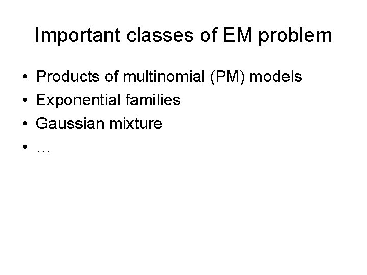
Important classes of EM problem • • Products of multinomial (PM) models Exponential families Gaussian mixture …

The EM algorithm for PM models

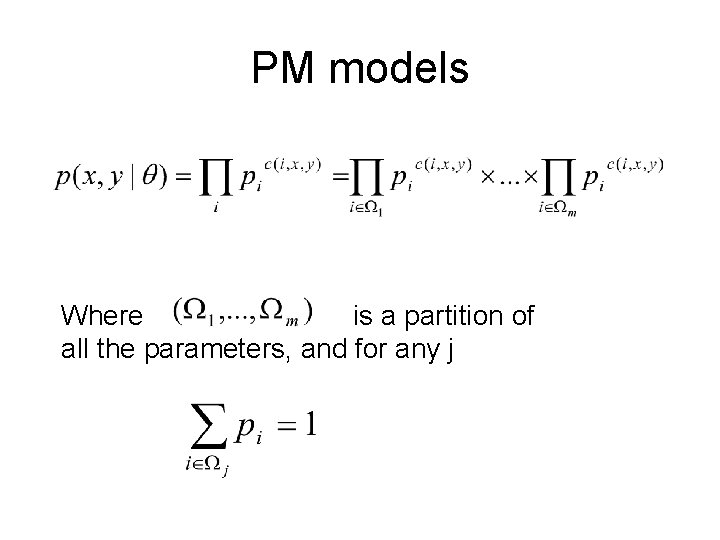
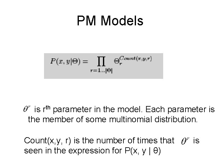
PM models Where is a partition of all the parameters, and for any j

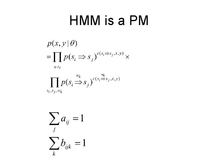
HMM is a PM

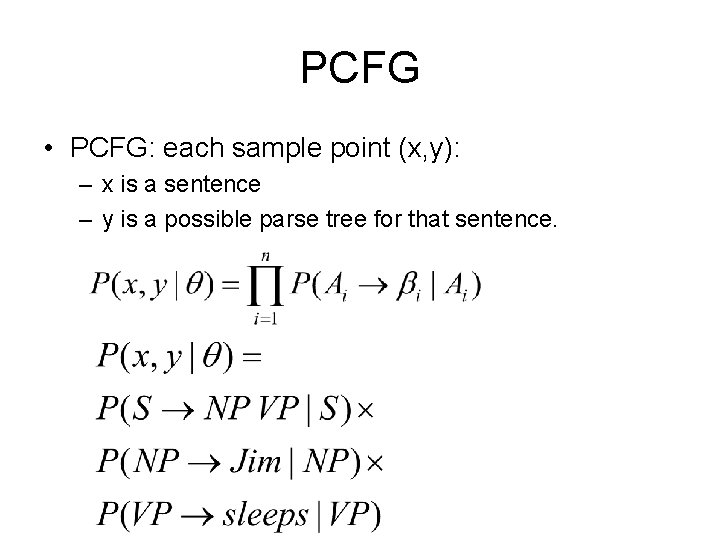
PCFG • PCFG: each sample point (x, y): – x is a sentence – y is a possible parse tree for that sentence.

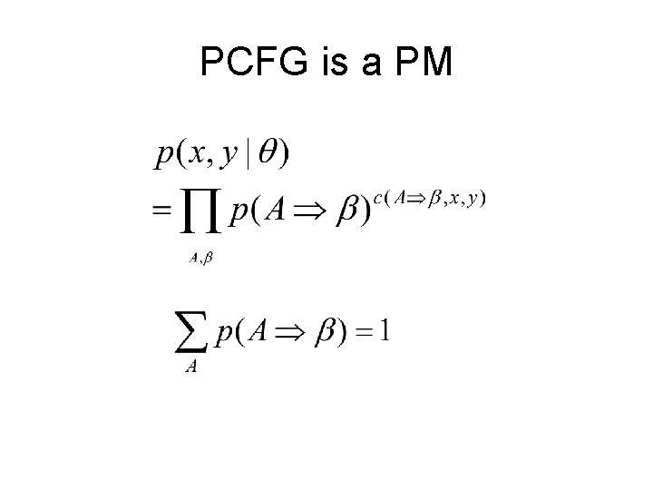
PCFG is a PM

Q-function for PM

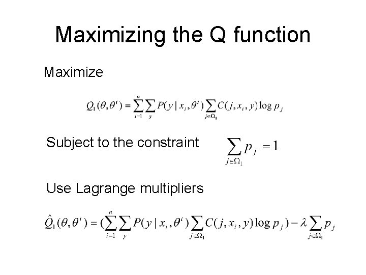
Maximizing the Q function Maximize Subject to the constraint Use Lagrange multipliers

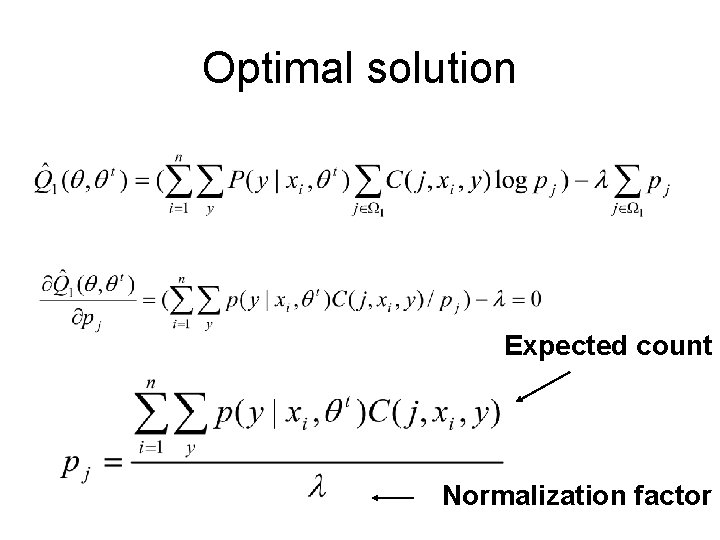
Optimal solution Expected count Normalization factor

PM Models is rth parameter in the model. Each parameter is the member of some multinomial distribution. Count(x, y, r) is the number of times that seen in the expression for P(x, y | θ) is

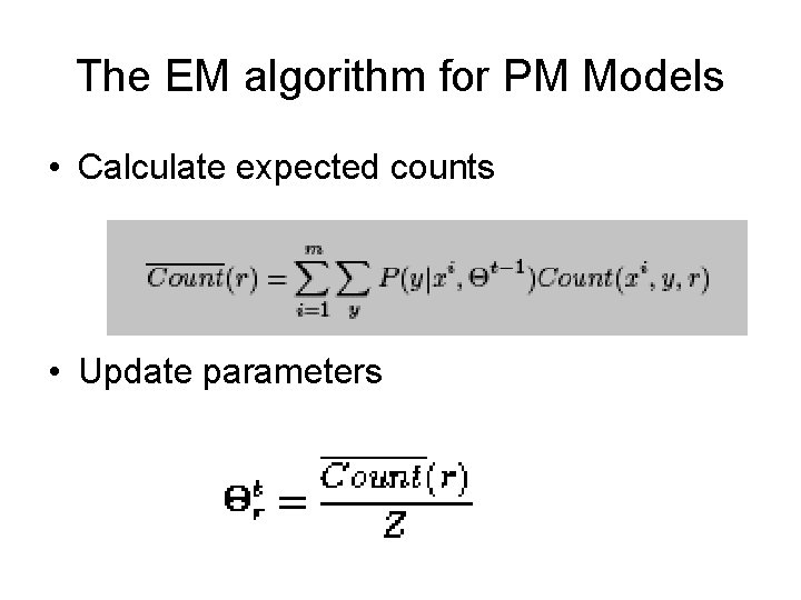
The EM algorithm for PM Models • Calculate expected counts • Update parameters

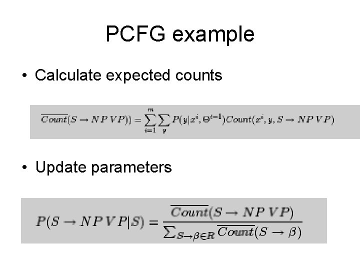
PCFG example • Calculate expected counts • Update parameters

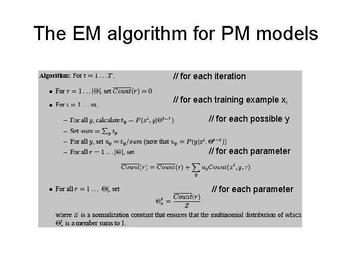
The EM algorithm for PM models // for each iteration // for each training example xi // for each possible y // for each parameter

Inside-outside algorithm

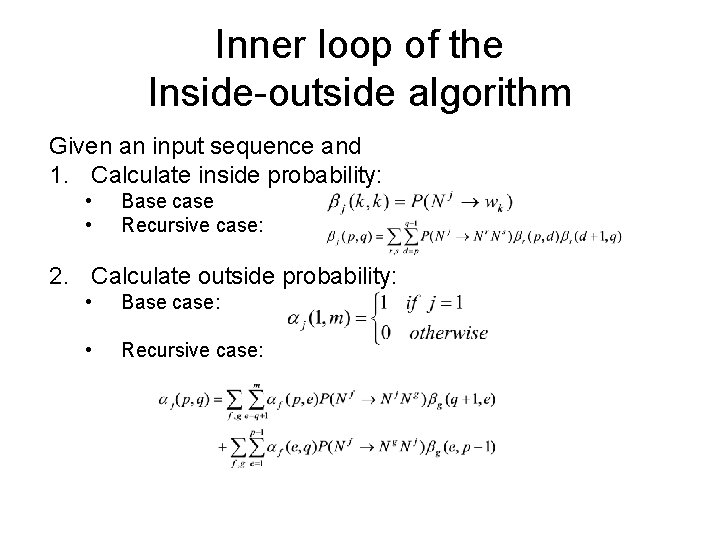
Inner loop of the Inside-outside algorithm Given an input sequence and 1. Calculate inside probability: • • Base case Recursive case: 2. Calculate outside probability: • Base case: • Recursive case:

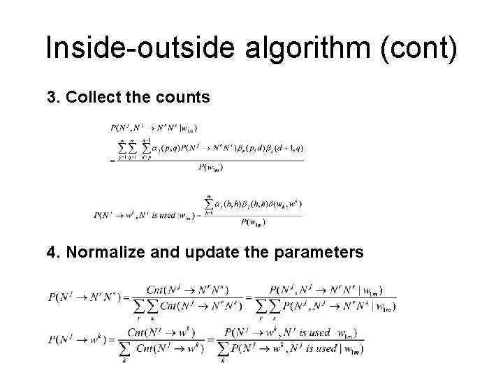
Inside-outside algorithm (cont) 3. Collect the counts 4. Normalize and update the parameters

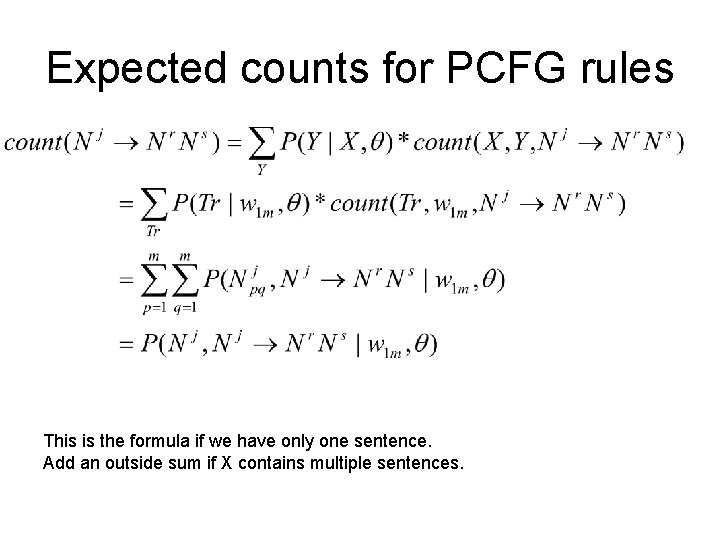
Expected counts for PCFG rules This is the formula if we have only one sentence. Add an outside sum if X contains multiple sentences.

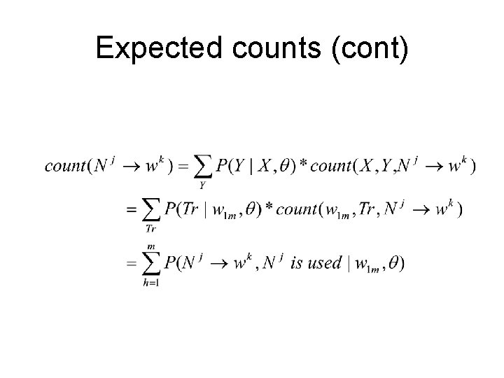
Expected counts (cont)

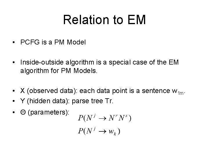
Relation to EM • PCFG is a PM Model • Inside-outside algorithm is a special case of the EM algorithm for PM Models. • X (observed data): each data point is a sentence w 1 m. • Y (hidden data): parse tree Tr. • Θ (parameters):

Forward-backward algorithm

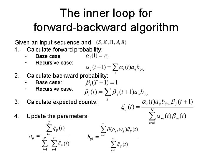
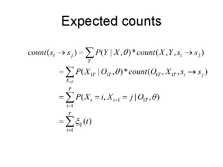
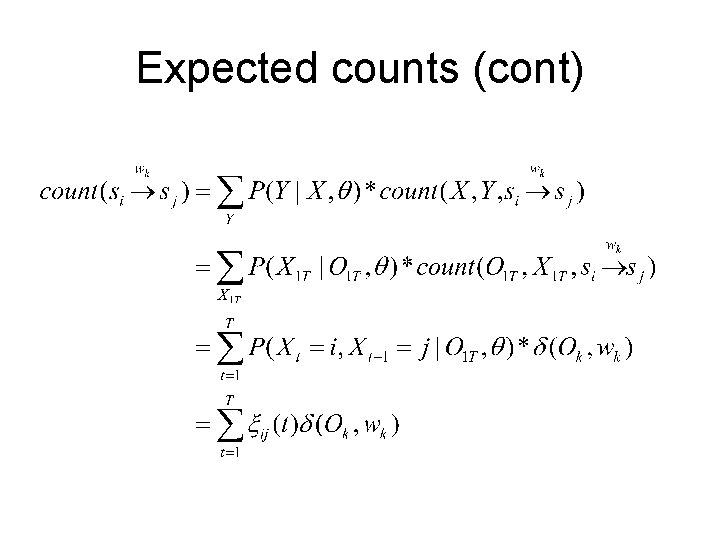
The inner loop forward-backward algorithm Given an input sequence and 1. Calculate forward probability: • • 2. Base case Recursive case: Calculate backward probability: • • Base case: Recursive case: 3. Calculate expected counts: 4. Update the parameters:

Expected counts

Expected counts (cont)

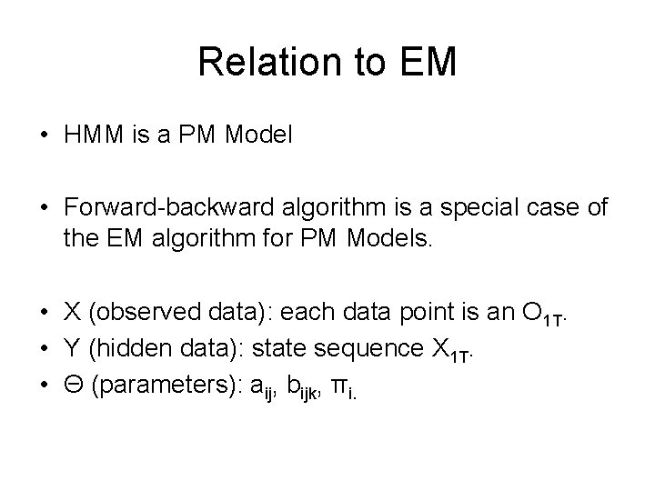
Relation to EM • HMM is a PM Model • Forward-backward algorithm is a special case of the EM algorithm for PM Models. • X (observed data): each data point is an O 1 T. • Y (hidden data): state sequence X 1 T. • Θ (parameters): aij, bijk, πi.

IBM models for MT

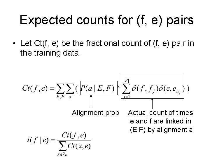
Expected counts for (f, e) pairs • Let Ct(f, e) be the fractional count of (f, e) pair in the training data. Alignment prob Actual count of times e and f are linked in (E, F) by alignment a

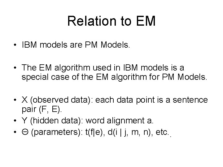
Relation to EM • IBM models are PM Models. • The EM algorithm used in IBM models is a special case of the EM algorithm for PM Models. • X (observed data): each data point is a sentence pair (F, E). • Y (hidden data): word alignment a. • Θ (parameters): t(f|e), d(i | j, m, n), etc. .

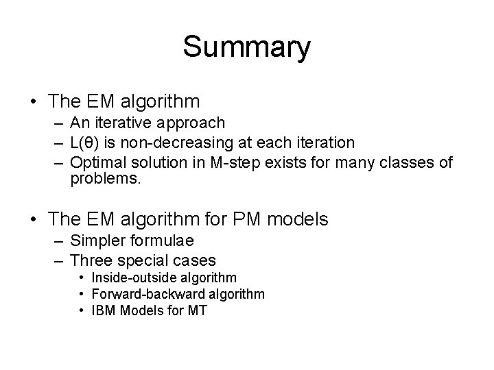
Summary • The EM algorithm – An iterative approach – L(θ) is non-decreasing at each iteration – Optimal solution in M-step exists for many classes of problems. • The EM algorithm for PM models – Simpler formulae – Three special cases • Inside-outside algorithm • Forward-backward algorithm • IBM Models for MT

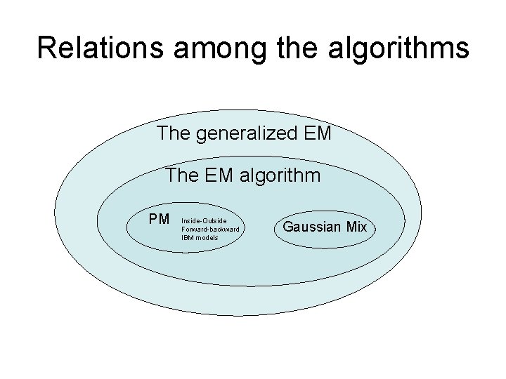
Relations among the algorithms The generalized EM The EM algorithm PM Inside-Outside Forward-backward IBM models Gaussian Mix

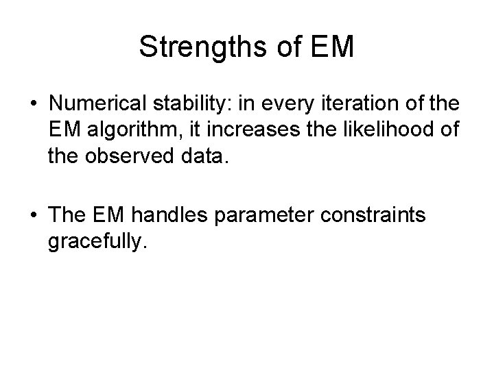
Strengths of EM • Numerical stability: in every iteration of the EM algorithm, it increases the likelihood of the observed data. • The EM handles parameter constraints gracefully.

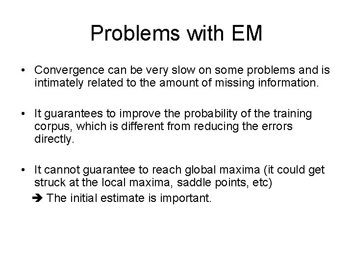
Problems with EM • Convergence can be very slow on some problems and is intimately related to the amount of missing information. • It guarantees to improve the probability of the training corpus, which is different from reducing the errors directly. • It cannot guarantee to reach global maxima (it could get struck at the local maxima, saddle points, etc) The initial estimate is important.

Additional slides

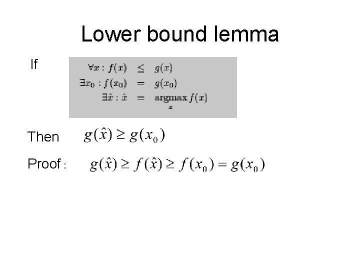
Lower bound lemma If Then Proof :

L(θ) is non-decreasing Let We have (By lower bound lemma)