Elementary Statistics Picturing The World Sixth Edition Chapter

Elementary Statistics: Picturing The World Sixth Edition Chapter 5 Normal Probability Distributions Copyright © 2015, 2012, 2009 Pearson Education, Inc. All Rights Reserved

Chapter Outline 5. 1 introduction to Normal Distributions and the standard Normal Distributions 5. 2 Normal Distributions: Finding probabilities 5. 3 Normal Distributions: Finding Values 5. 4 Sampling Distributions and the Central Limit Theorem 5. 5 Normal approximations to binomial Distributions Copyright © 2015, 2012, 2009 Pearson Education, Inc. All Rights Reserved

Section 5. 1 Introduction to Normal Distributions and the Standard Normal Distributions Copyright © 2015, 2012, 2009 Pearson Education, Inc. All Rights Reserved

Section 5. 1 Objectives • How to interpret graphs of normal probability distributions • How to find areas under the standard normal curve Copyright © 2015, 2012, 2009 Pearson Education, Inc. All Rights Reserved

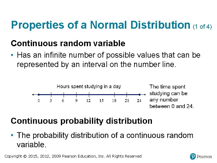
Properties of a Normal Distribution (1 of 4) Continuous random variable • Has an infinite number of possible values that can be represented by an interval on the number line. Copyright © 2015, 2012, 2009 Pearson Education, Inc. All Rights Reserved

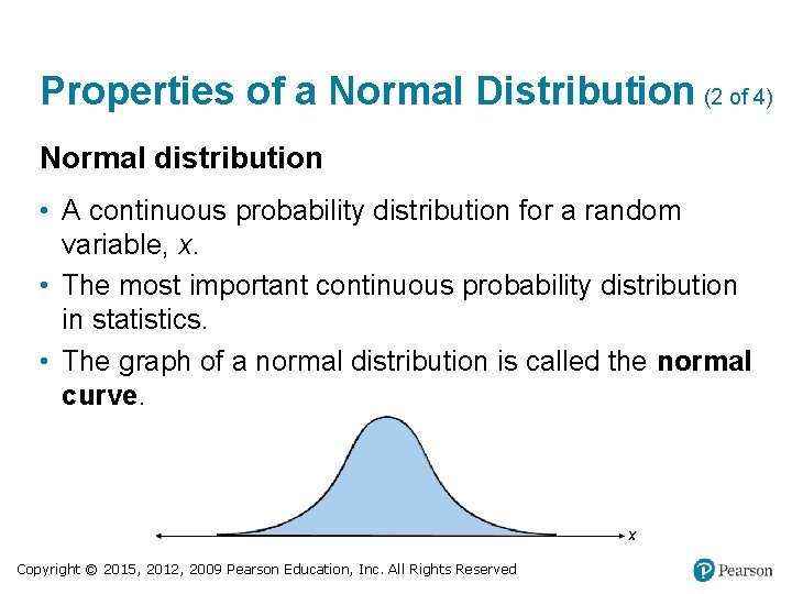
Properties of a Normal Distribution (2 of 4) Normal distribution • A continuous probability distribution for a random variable, x. • The most important continuous probability distribution in statistics. • The graph of a normal distribution is called the normal curve. Copyright © 2015, 2012, 2009 Pearson Education, Inc. All Rights Reserved

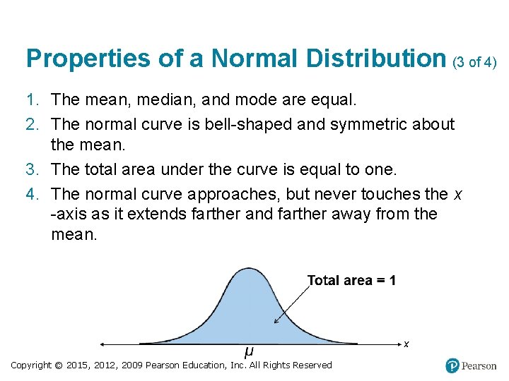
Properties of a Normal Distribution (3 of 4) 1. The mean, median, and mode are equal. 2. The normal curve is bell-shaped and symmetric about the mean. 3. The total area under the curve is equal to one. 4. The normal curve approaches, but never touches the x -axis as it extends farther and farther away from the mean. Copyright © 2015, 2012, 2009 Pearson Education, Inc. All Rights Reserved

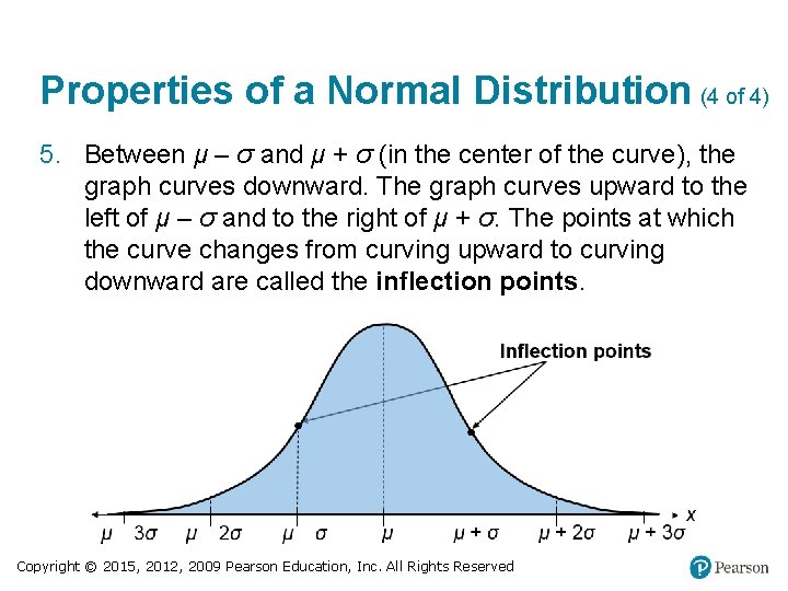
Properties of a Normal Distribution (4 of 4) 5. Between μ – σ and μ + σ (in the center of the curve), the graph curves downward. The graph curves upward to the left of μ – σ and to the right of μ + σ. The points at which the curve changes from curving upward to curving downward are called the inflection points. Copyright © 2015, 2012, 2009 Pearson Education, Inc. All Rights Reserved

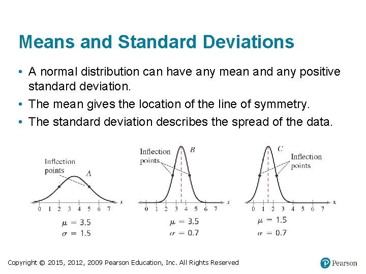
Means and Standard Deviations • A normal distribution can have any mean and any positive standard deviation. • The mean gives the location of the line of symmetry. • The standard deviation describes the spread of the data. Copyright © 2015, 2012, 2009 Pearson Education, Inc. All Rights Reserved

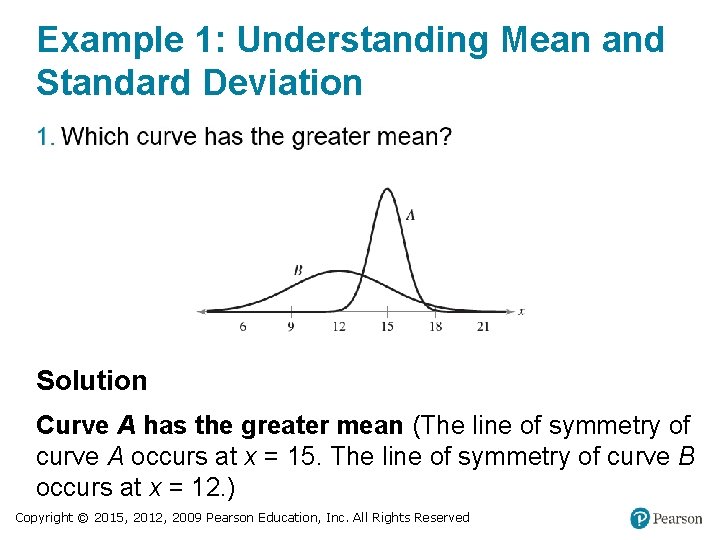
Example 1: Understanding Mean and Standard Deviation Solution Curve A has the greater mean (The line of symmetry of curve A occurs at x = 15. The line of symmetry of curve B occurs at x = 12. ) Copyright © 2015, 2012, 2009 Pearson Education, Inc. All Rights Reserved

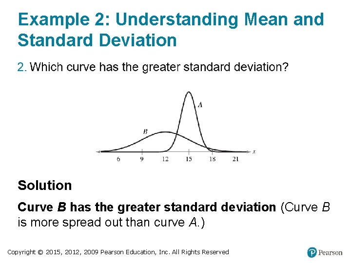
Example 2: Understanding Mean and Standard Deviation Solution Curve B has the greater standard deviation (Curve B is more spread out than curve A. ) Copyright © 2015, 2012, 2009 Pearson Education, Inc. All Rights Reserved

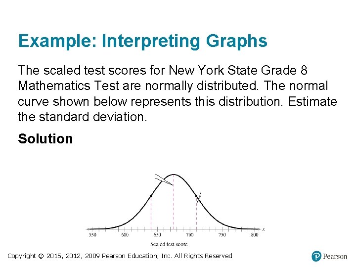
Example: Interpreting Graphs The scaled test scores for New York State Grade 8 Mathematics Test are normally distributed. The normal curve shown below represents this distribution. Estimate the standard deviation. Solution Copyright © 2015, 2012, 2009 Pearson Education, Inc. All Rights Reserved

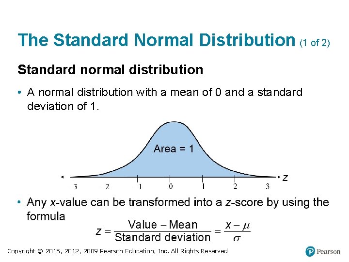
The Standard Normal Distribution (1 of 2) Standard normal distribution • A normal distribution with a mean of 0 and a standard deviation of 1. Copyright © 2015, 2012, 2009 Pearson Education, Inc. All Rights Reserved

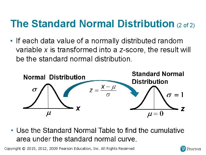
The Standard Normal Distribution (2 of 2) • If each data value of a normally distributed random variable x is transformed into a z-score, the result will be the standard normal distribution. Copyright © 2015, 2012, 2009 Pearson Education, Inc. All Rights Reserved

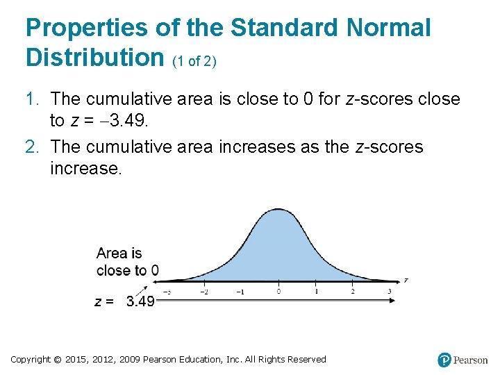
Properties of the Standard Normal Distribution (1 of 2) 1. The cumulative area is close to 0 for z-scores close to z = 3. 49. 2. The cumulative area increases as the z-scores increase. Copyright © 2015, 2012, 2009 Pearson Education, Inc. All Rights Reserved

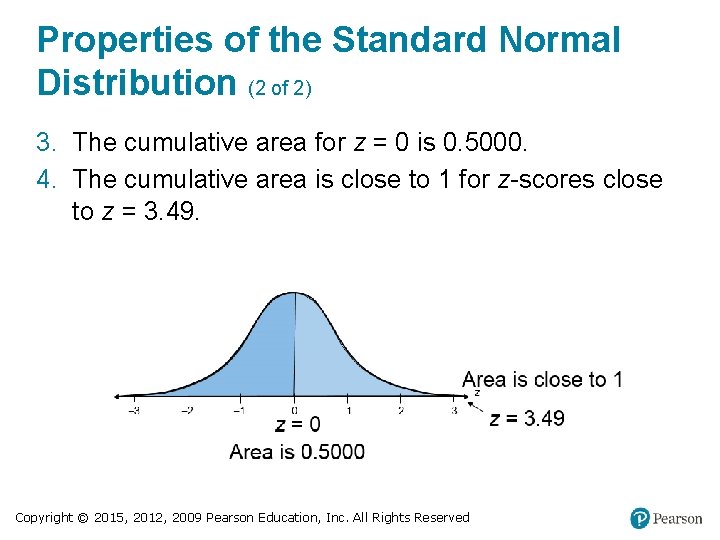
Properties of the Standard Normal Distribution (2 of 2) 3. The cumulative area for z = 0 is 0. 5000. 4. The cumulative area is close to 1 for z-scores close to z = 3. 49. Copyright © 2015, 2012, 2009 Pearson Education, Inc. All Rights Reserved

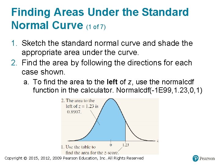
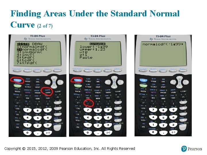
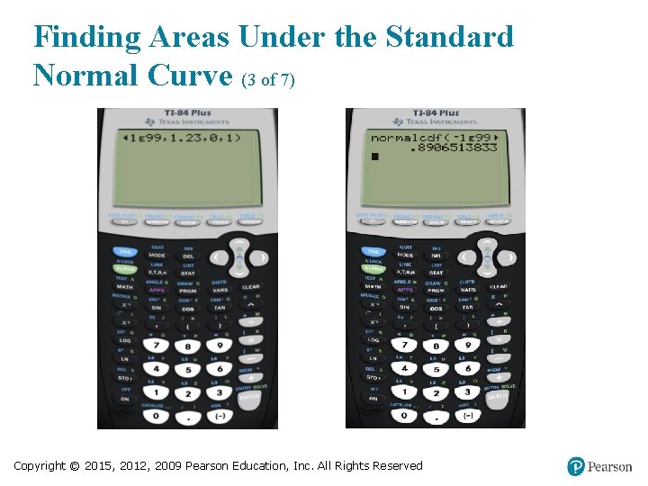
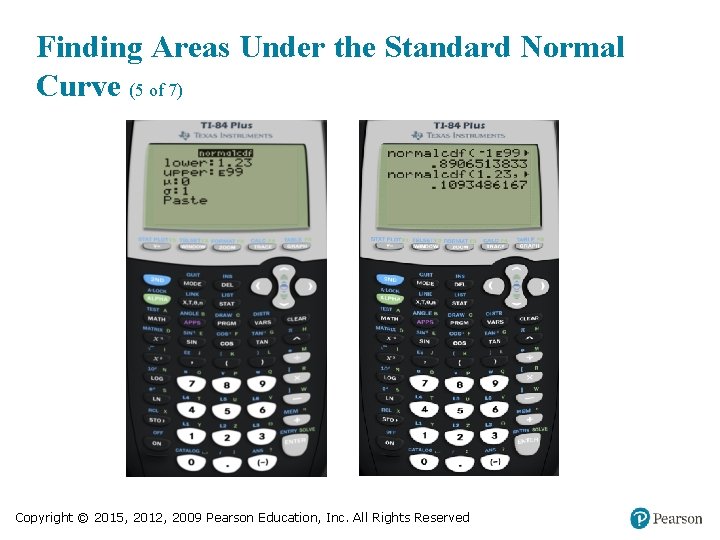
Finding Areas Under the Standard Normal Curve (1 of 7) 1. Sketch the standard normal curve and shade the appropriate area under the curve. 2. Find the area by following the directions for each case shown. a. To find the area to the left of z, use the normalcdf function in the calculator. Normalcdf(-1 E 99, 1. 23, 0, 1) Copyright © 2015, 2012, 2009 Pearson Education, Inc. All Rights Reserved

Finding Areas Under the Standard Normal Curve (2 of 7) Copyright © 2015, 2012, 2009 Pearson Education, Inc. All Rights Reserved

Finding Areas Under the Standard Normal Curve (3 of 7) Copyright © 2015, 2012, 2009 Pearson Education, Inc. All Rights Reserved

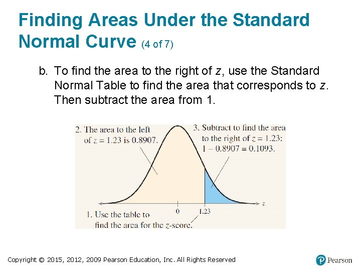
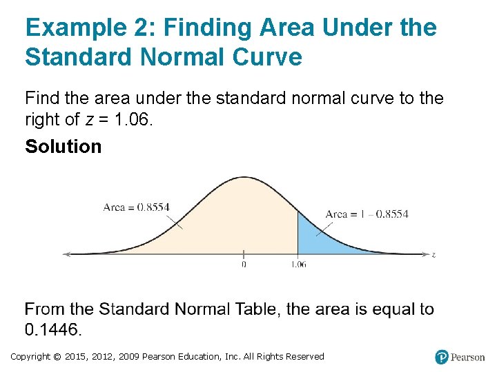
Finding Areas Under the Standard Normal Curve (4 of 7) b. To find the area to the right of z, use the Standard Normal Table to find the area that corresponds to z. Then subtract the area from 1. Copyright © 2015, 2012, 2009 Pearson Education, Inc. All Rights Reserved

Finding Areas Under the Standard Normal Curve (5 of 7) Copyright © 2015, 2012, 2009 Pearson Education, Inc. All Rights Reserved

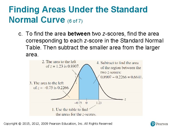
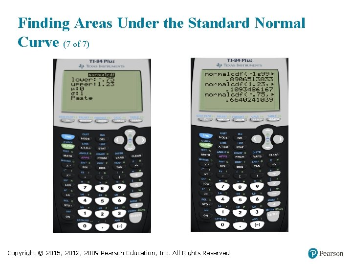
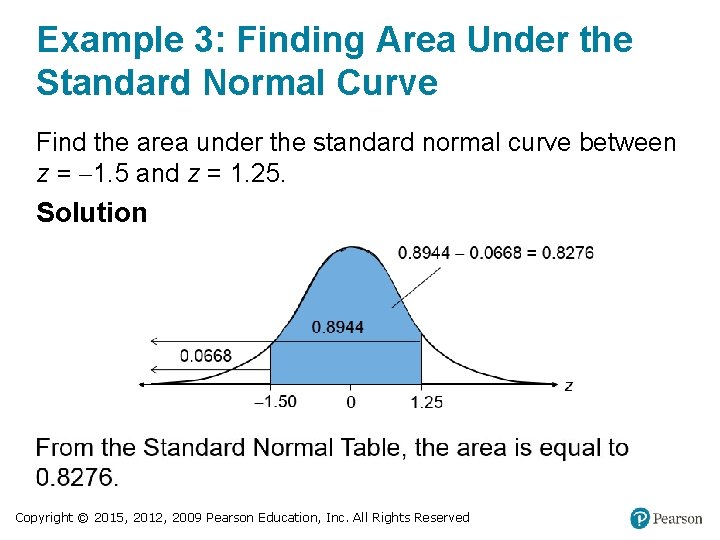
Finding Areas Under the Standard Normal Curve (6 of 7) c. To find the area between two z-scores, find the area corresponding to each z-score in the Standard Normal Table. Then subtract the smaller area from the larger area. Copyright © 2015, 2012, 2009 Pearson Education, Inc. All Rights Reserved

Finding Areas Under the Standard Normal Curve (7 of 7) Copyright © 2015, 2012, 2009 Pearson Education, Inc. All Rights Reserved

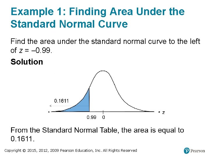
Example 1: Finding Area Under the Standard Normal Curve Find the area under the standard normal curve to the left of z = – 0. 99. Solution Copyright © 2015, 2012, 2009 Pearson Education, Inc. All Rights Reserved

Example 2: Finding Area Under the Standard Normal Curve Find the area under the standard normal curve to the right of z = 1. 06. Solution Copyright © 2015, 2012, 2009 Pearson Education, Inc. All Rights Reserved

Example 3: Finding Area Under the Standard Normal Curve Find the area under the standard normal curve between z = 1. 5 and z = 1. 25. Solution Copyright © 2015, 2012, 2009 Pearson Education, Inc. All Rights Reserved

Section 5. 1 Summary • Interpreted graphs of normal probability distributions • Found areas under the standard normal curve Copyright © 2015, 2012, 2009 Pearson Education, Inc. All Rights Reserved