Elementary Statistics Math 145 May 25 2010 Statistics

Elementary Statistics (Math 145) May 25, 2010

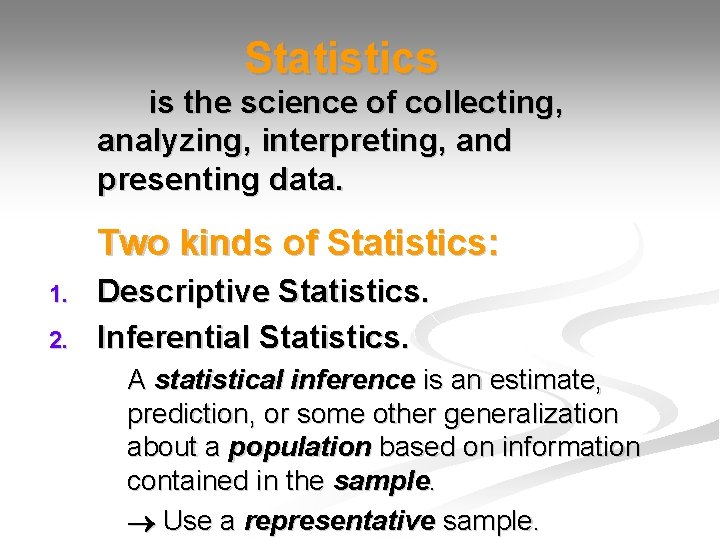
Statistics is the science of collecting, analyzing, interpreting, and presenting data. Two kinds of Statistics: 1. 2. Descriptive Statistics. Inferential Statistics. A statistical inference is an estimate, prediction, or some other generalization about a population based on information contained in the sample. Use a representative sample.

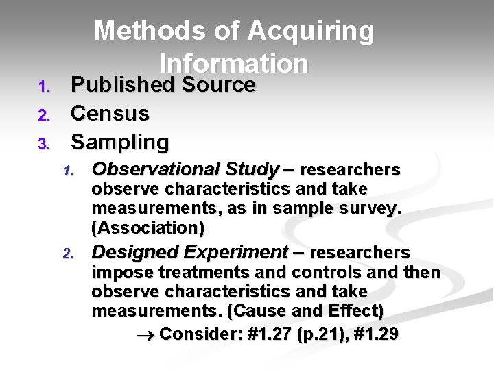
1. 2. 3. Methods of Acquiring Information Published Source Census Sampling 1. 2. Observational Study – researchers observe characteristics and take measurements, as in sample survey. (Association) Designed Experiment – researchers impose treatments and controls and then observe characteristics and take measurements. (Cause and Effect) Consider: #1. 27 (p. 21), #1. 29

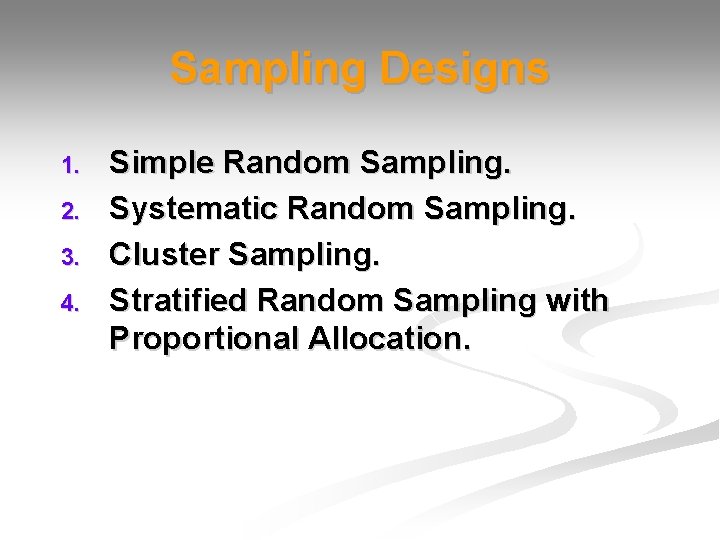
Sampling Designs 1. 2. 3. 4. Simple Random Sampling. Systematic Random Sampling. Cluster Sampling. Stratified Random Sampling with Proportional Allocation.

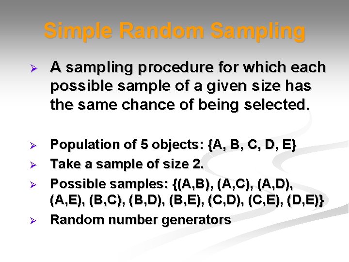
Simple Random Sampling Ø A sampling procedure for which each possible sample of a given size has the same chance of being selected. Ø Population of 5 objects: {A, B, C, D, E} Take a sample of size 2. Possible samples: {(A, B), (A, C), (A, D), (A, E), (B, C), (B, D), (B, E), (C, D), (C, E), (D, E)} Random number generators Ø Ø Ø

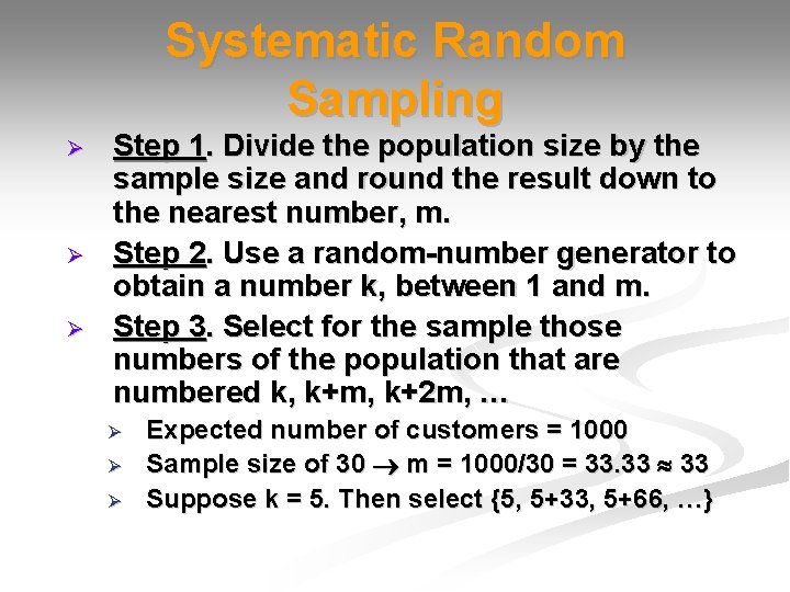
Systematic Random Sampling Ø Ø Ø Step 1. Divide the population size by the sample size and round the result down to the nearest number, m. Step 2. Use a random-number generator to obtain a number k, between 1 and m. Step 3. Select for the sample those numbers of the population that are numbered k, k+m, k+2 m, … Ø Ø Ø Expected number of customers = 1000 Sample size of 30 m = 1000/30 = 33. 33 Suppose k = 5. Then select {5, 5+33, 5+66, …}

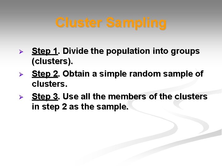
Cluster Sampling Ø Ø Ø Step 1. Divide the population into groups (clusters). Step 2. Obtain a simple random sample of clusters. Step 3. Use all the members of the clusters in step 2 as the sample.

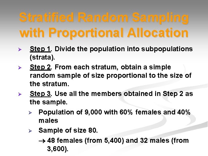
Stratified Random Sampling with Proportional Allocation Ø Ø Ø Step 1. Divide the population into subpopulations (strata). Step 2. From each stratum, obtain a simple random sample of size proportional to the size of the stratum. Step 3. Use all the members obtained in Step 2 as the sample. Ø Population of 9, 000 with 60% females and 40% males Ø Sample of size 80. 48 females (from 5, 400) and 32 males (from 3, 600).

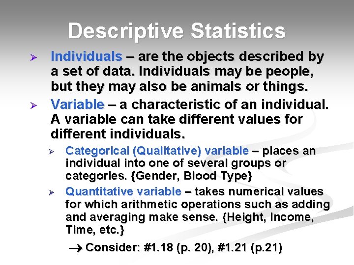
Descriptive Statistics Ø Ø Individuals – are the objects described by a set of data. Individuals may be people, but they may also be animals or things. Variable – a characteristic of an individual. A variable can take different values for different individuals. Ø Ø Categorical (Qualitative) variable – places an individual into one of several groups or categories. {Gender, Blood Type} Quantitative variable – takes numerical values for which arithmetic operations such as adding and averaging make sense. {Height, Income, Time, etc. } Consider: #1. 18 (p. 20), #1. 21 (p. 21)

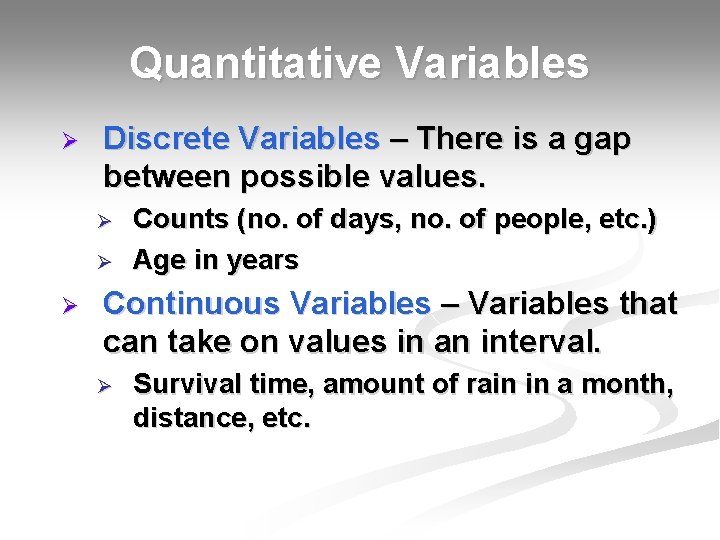
Quantitative Variables Ø Discrete Variables – There is a gap between possible values. Ø Ø Ø Counts (no. of days, no. of people, etc. ) Age in years Continuous Variables – Variables that can take on values in an interval. Ø Survival time, amount of rain in a month, distance, etc.

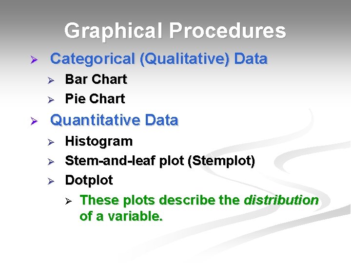
Graphical Procedures Ø Categorical (Qualitative) Data Ø Ø Ø Bar Chart Pie Chart Quantitative Data Ø Ø Ø Histogram Stem-and-leaf plot (Stemplot) Dotplot Ø These plots describe the distribution of a variable.

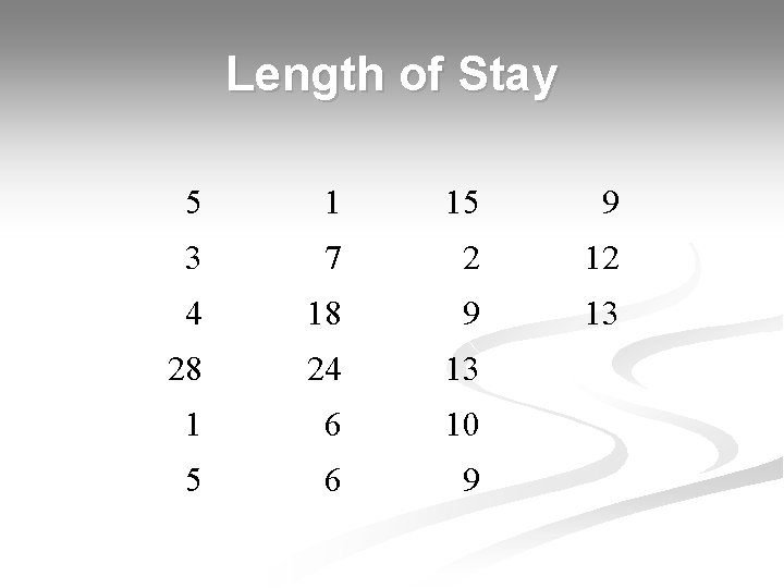
Length of Stay 5 1 15 9 3 7 2 12 4 18 9 13 28 24 13 1 6 10 5 6 9

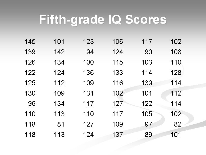
Fifth-grade IQ Scores 145 139 126 122 101 142 134 123 94 100 136 106 124 115 133 117 90 103 114 102 108 110 128 125 130 96 110 118 112 109 134 113 81 113 109 131 117 110 127 124 116 102 127 117 109 137 139 101 122 105 97 89 114 112 114 102 82 101

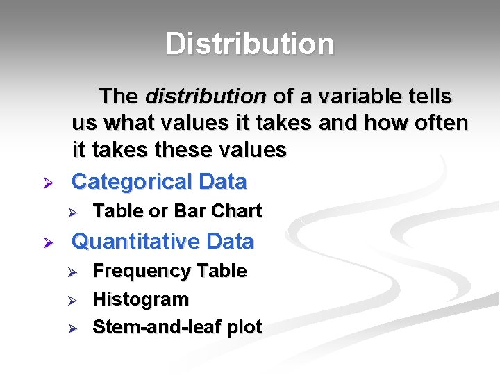
Distribution Ø The distribution of a variable tells us what values it takes and how often it takes these values Categorical Data Ø Ø Table or Bar Chart Quantitative Data Ø Ø Ø Frequency Table Histogram Stem-and-leaf plot

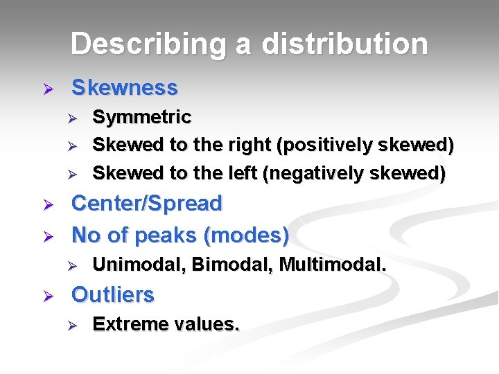
Describing a distribution Ø Skewness Ø Ø Ø Center/Spread No of peaks (modes) Ø Ø Symmetric Skewed to the right (positively skewed) Skewed to the left (negatively skewed) Unimodal, Bimodal, Multimodal. Outliers Ø Extreme values.

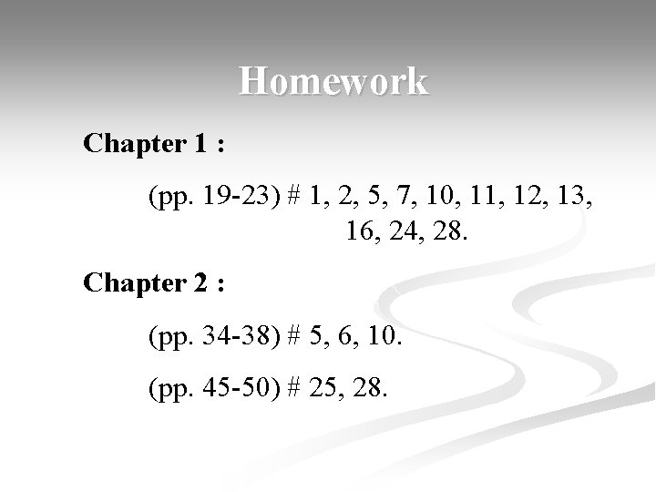
Homework Chapter 1 : (pp. 19 -23) # 1, 2, 5, 7, 10, 11, 12, 13, 16, 24, 28. Chapter 2 : (pp. 34 -38) # 5, 6, 10. (pp. 45 -50) # 25, 28.