Electromechanical systems Motors DC motors Induction motors Variable

Electromechanical systems • Motors – DC motors – Induction motors – Variable reluctance motors • • Generators Angular position sensors Encoders Tachometers

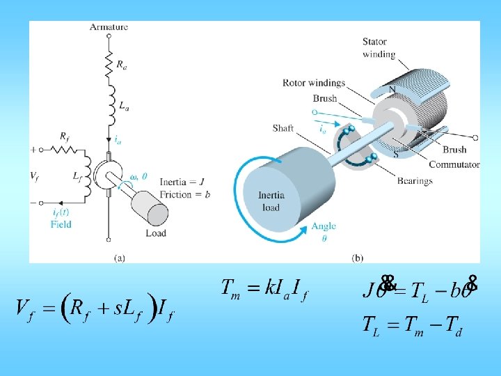
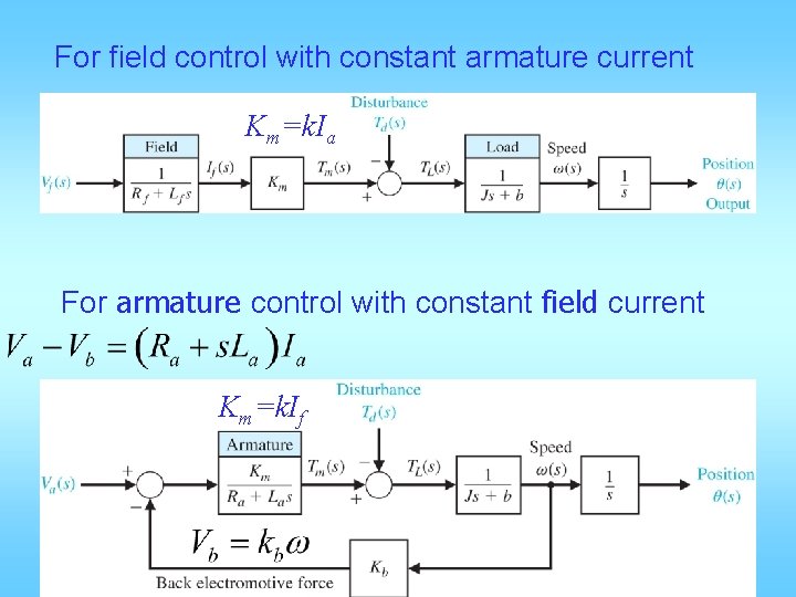
For field control with constant armature current Km=k. Ia For armature control with constant field current Km=k. If

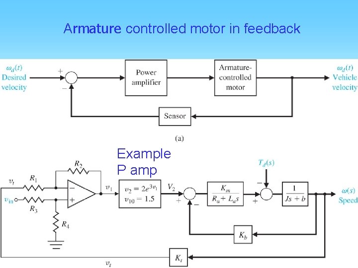
Armature controlled motor in feedback Example P amp

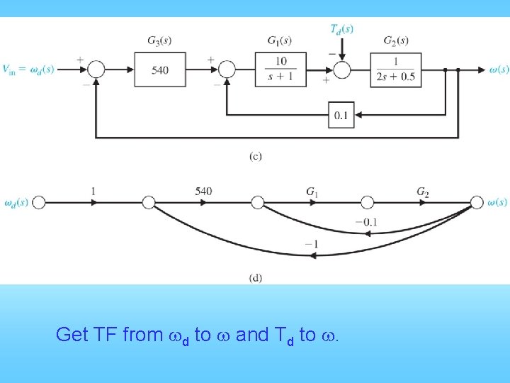
Get TF from wd to w and Td to w.

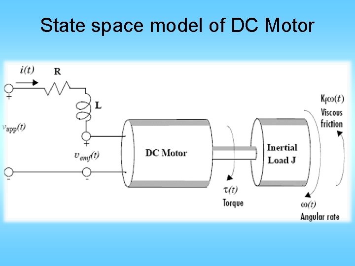
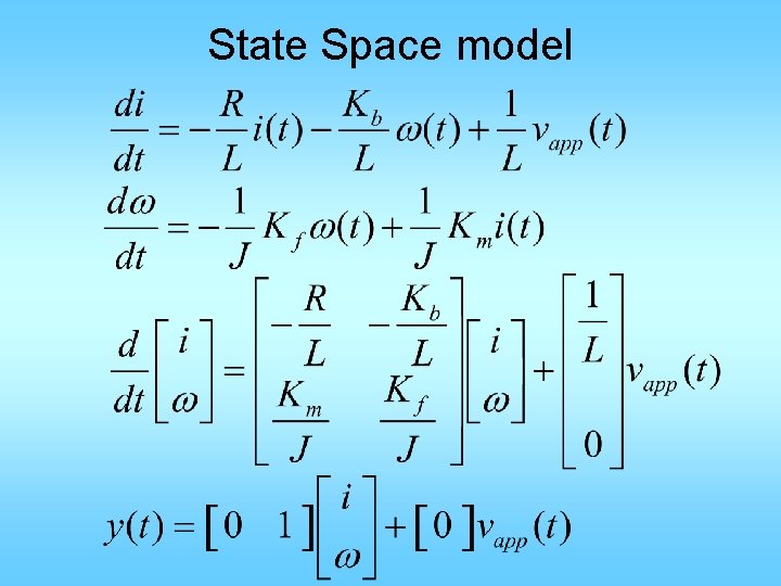
State space model of DC Motor

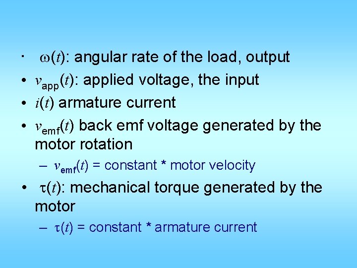
• • w(t): angular rate of the load, output vapp(t): applied voltage, the input i(t) armature current vemf(t) back emf voltage generated by the motor rotation – vemf(t) = constant * motor velocity • t(t): mechanical torque generated by the motor – t(t) = constant * armature current

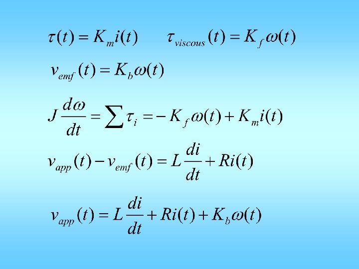
State Space model

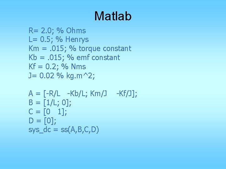
Matlab R= 2. 0; % Ohms L= 0. 5; % Henrys Km =. 015; % torque constant Kb =. 015; % emf constant Kf = 0. 2; % Nms J= 0. 02 % kg. m^2; A = [-R/L -Kb/L; Km/J B = [1/L; 0]; C = [0 1]; D = [0]; sys_dc = ss(A, B, C, D) -Kf/J];

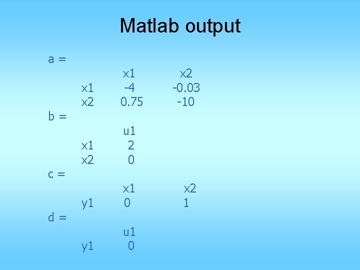
Matlab output a= b= c= d= x 1 x 2 x 1 -4 0. 75 x 1 x 2 u 1 2 0 y 1 x 1 0 y 1 u 1 0 x 2 -0. 03 -10 x 2 1

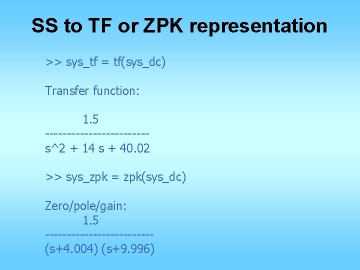
SS to TF or ZPK representation >> sys_tf = tf(sys_dc) Transfer function: 1. 5 ------------s^2 + 14 s + 40. 02 >> sys_zpk = zpk(sys_dc) Zero/pole/gain: 1. 5 ------------(s+4. 004) (s+9. 996)

• Note: The state-space representation is best suited for numerical computations. For highest accuracy, convert to state space prior to combining models and avoid the transfer function and zero/pole/gain representations, except for model specification and inspection.

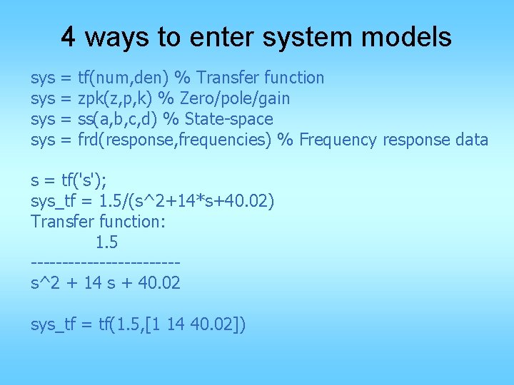
4 ways to enter system models sys sys = = tf(num, den) % Transfer function zpk(z, p, k) % Zero/pole/gain ss(a, b, c, d) % State-space frd(response, frequencies) % Frequency response data s = tf('s'); sys_tf = 1. 5/(s^2+14*s+40. 02) Transfer function: 1. 5 ------------s^2 + 14 s + 40. 02 sys_tf = tf(1. 5, [1 14 40. 02])

4 ways to enter system model sys_zpk = zpk([], [-9. 996 -4. 004], 1. 5) Zero/pole/gain: 1. 5 ------------(s+9. 996) (s+4. 004)

>> n=[1 2 3]; d=[1 4 5 6]; >> [A, B, C, D]=tf 2 ss(n, d) • In Matlab: >> A=[0 1; -2 -3]; >> B=[0; 1]; >> C=[1 3]; >> D=[0]; >> [n, d]=ss 2 tf(A, B, C, D) n= 0 d= 1 3. 0000 3 2 1. 0000 A= -4 1 0 -5 0 1 -6 0 0 2 3 B= 1 0 0 C= 1 D= 0 >> tf(n, d) Transfer function: s^2 + 2 s + 3 ----------s^3 + 4 s^2 + 5 s + 6

Summary of Background • Elements of a control system • Block diagram, and its simplification • Signal flow graph, and Mason’s gain rule • Modeling, modeling – Use math to describe system operation – Math eq from known physical laws – Circuits, linear motion, angular motion, and electromechanical system – ODE, SS, TF, zpk, FR

Coming up next • What is a good control system – Time domain specification • Transient, stability, steady state errors – Frequency domain specifications • Mid frequency, low freq, high freq, loop shape • How to make a system good – Root-locus based controller design – Frequency response design (loop shaping) – Two degree of freedom controller design – State feedback design, optimal control, nonlinear control, adaptive control, robust control