Eigenvalues and Eigenvectors Anxn has precisely n not

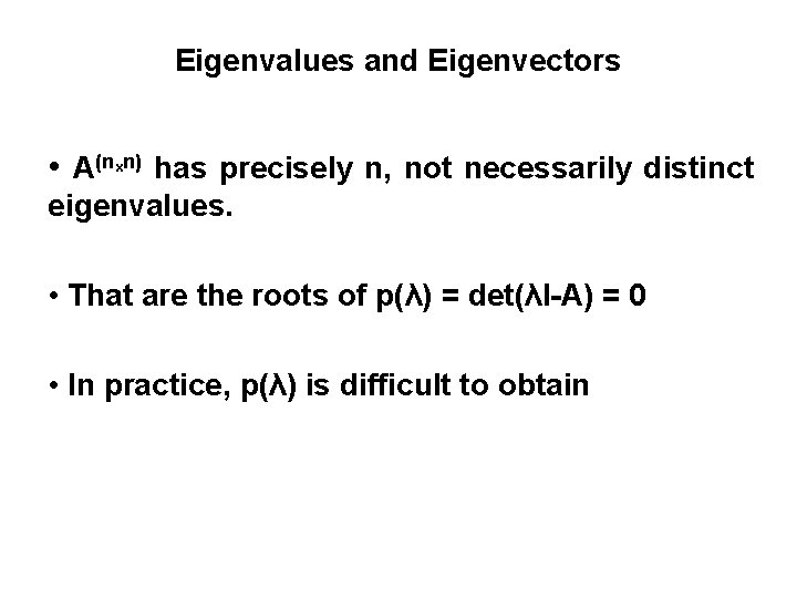
Eigenvalues and Eigenvectors • A(nxn) has precisely n, not necessarily distinct eigenvalues. • That are the roots of p(λ) = det(λI-A) = 0 • In practice, p(λ) is difficult to obtain

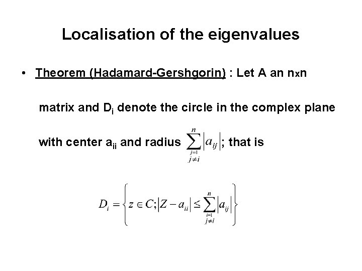
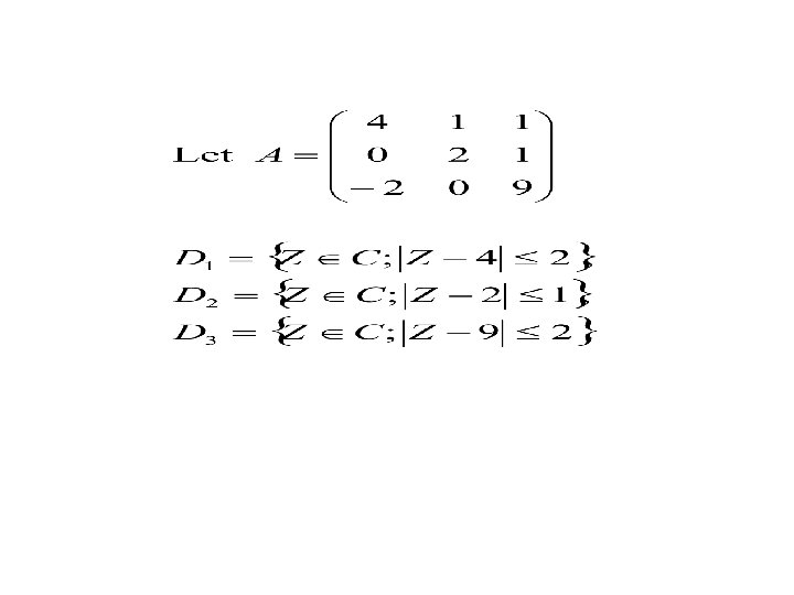
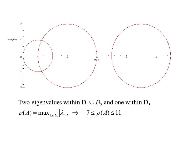
Localisation of the eigenvalues • Theorem (Hadamard-Gershgorin) : Let A an nxn matrix and Di denote the circle in the complex plane with center aii and radius ; that is

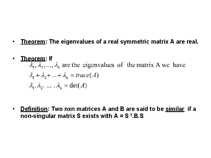
• Theorem: The eigenvalues of a real symmetric matrix A are real. • Theorem: If • Definition: Two nxn matrices A and B are said to be similar if a non-singular matrix S exists with A = S-1. B. S

• Theorem: Suppose A and B are similar nxn matrices and λ is an eigenvalue of A, with associated eigenvector X. Then λ is also an eigenvalue of B and if A =S-1 BS, then SX is an eigenvector associated with λ and the matrix B. • Definition:

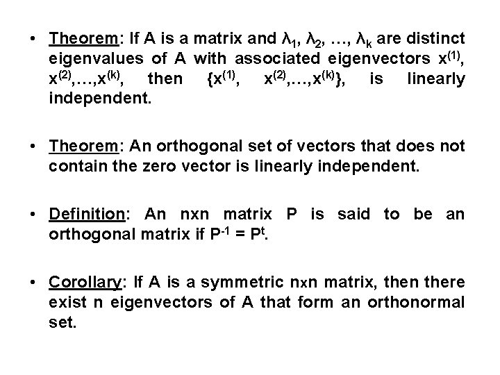
• Theorem: If A is a matrix and λ 1, λ 2, …, λk are distinct eigenvalues of A with associated eigenvectors x(1), x(2), …, x(k), then {x(1), x(2), …, x(k)}, is linearly independent. • Theorem: An orthogonal set of vectors that does not contain the zero vector is linearly independent. • Definition: An nxn matrix P is said to be an orthogonal matrix if P-1 = Pt. • Corollary: If A is a symmetric nxn matrix, then there exist n eigenvectors of A that form an orthonormal set.

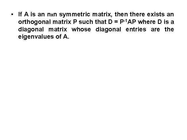
• If A is an nxn symmetric matrix, then there exists an orthogonal matrix P such that D = P-1 AP where D is a diagonal matrix whose diagonal entries are the eigenvalues of A.

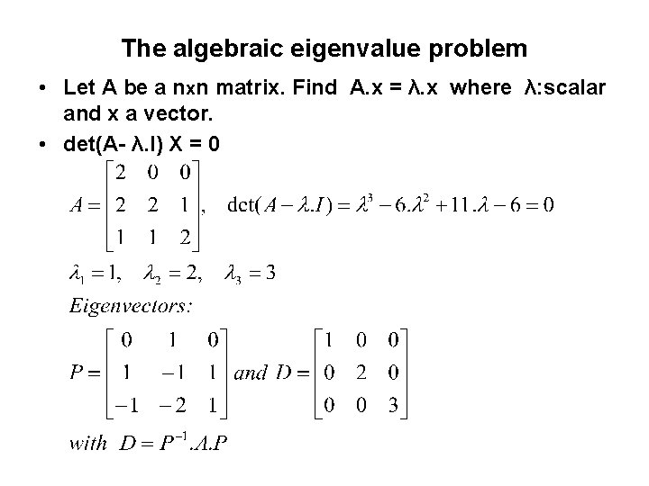
The algebraic eigenvalue problem • Let A be a nxn matrix. Find A. x = λ. x where λ: scalar and x a vector. • det(A- λ. I) X = 0

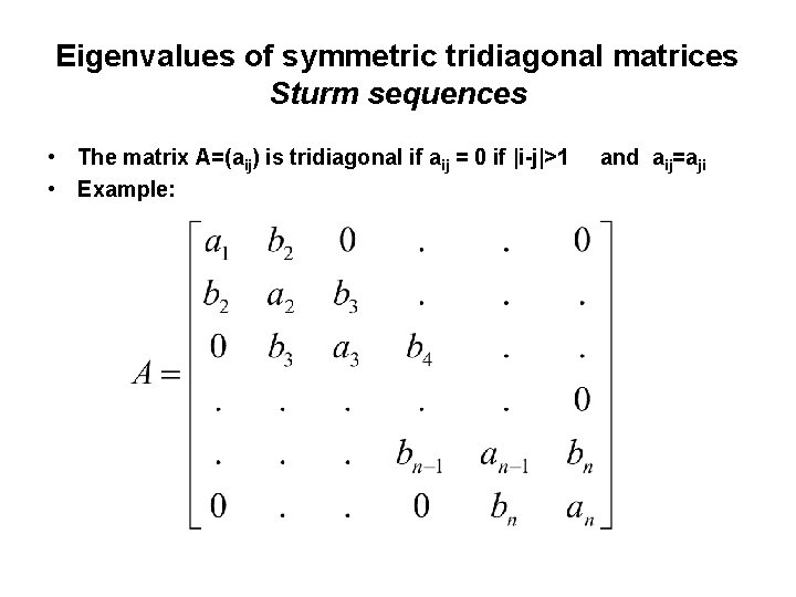
Eigenvalues of symmetric tridiagonal matrices Sturm sequences • The matrix A=(aij) is tridiagonal if aij = 0 if |i-j|>1 • Example: and aij=aji

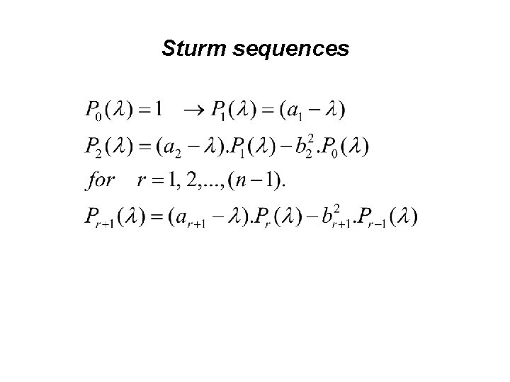
Sturm sequences

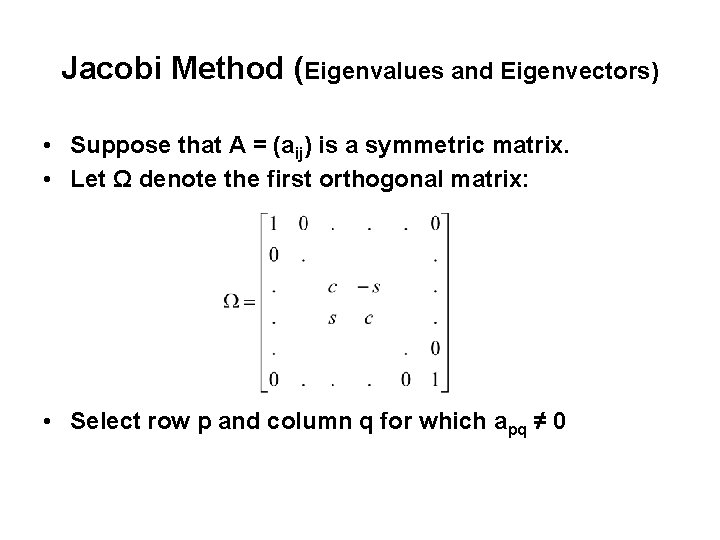
Jacobi Method (Eigenvalues and Eigenvectors) • Suppose that A = (aij) is a symmetric matrix. • Let Ω denote the first orthogonal matrix: • Select row p and column q for which apq ≠ 0

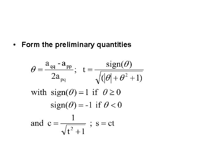
• Form the preliminary quantities

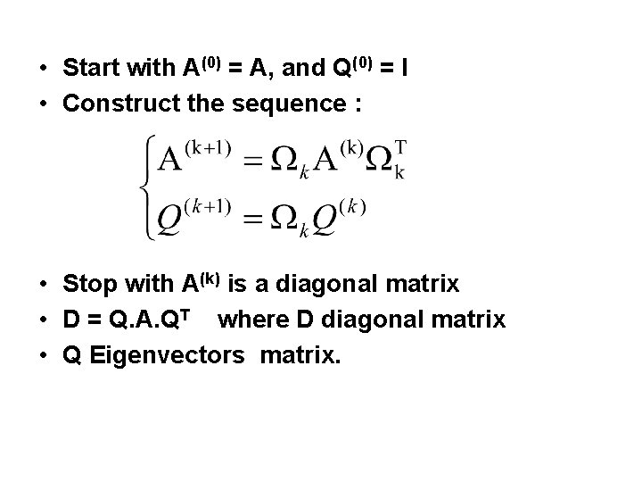
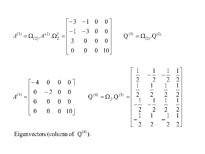
• Start with A(0) = A, and Q(0) = I • Construct the sequence : • Stop with A(k) is a diagonal matrix • D = Q. A. QT where D diagonal matrix • Q Eigenvectors matrix.

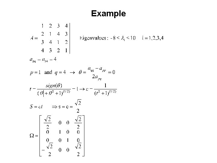
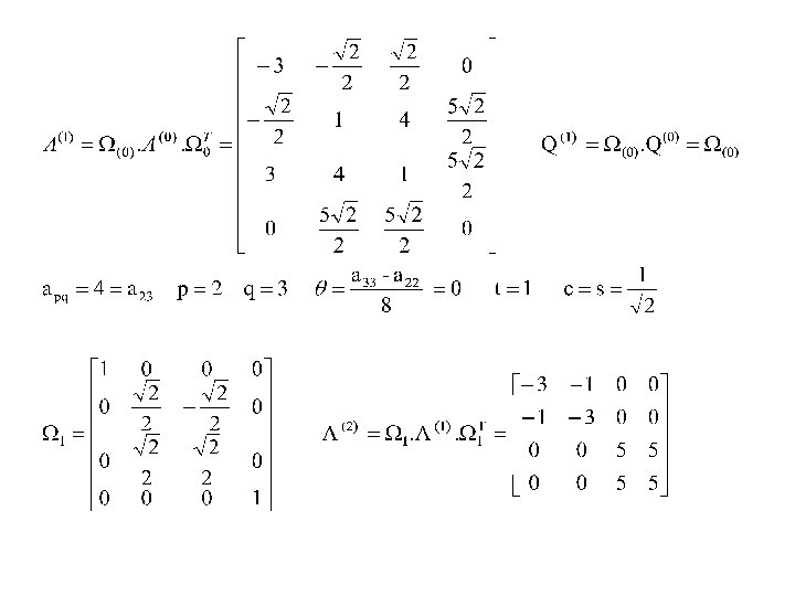
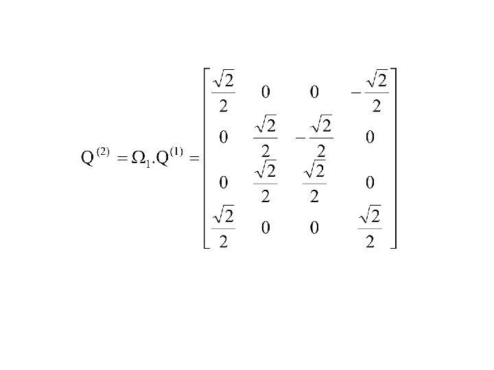
Example

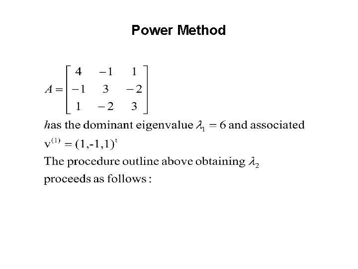
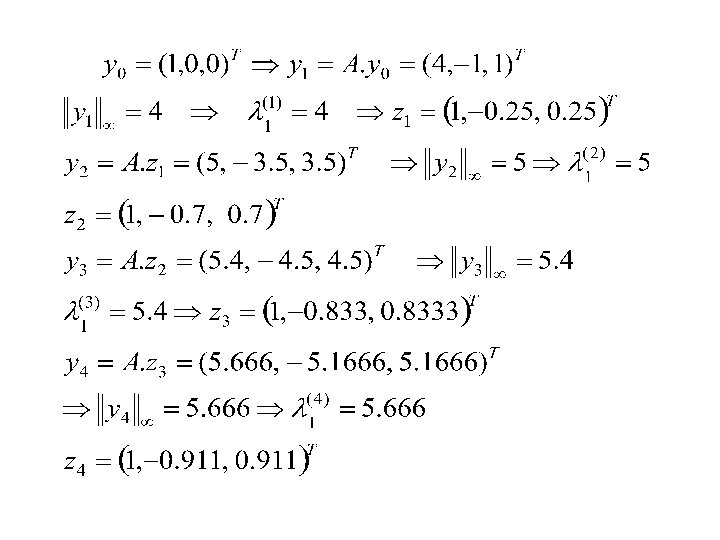
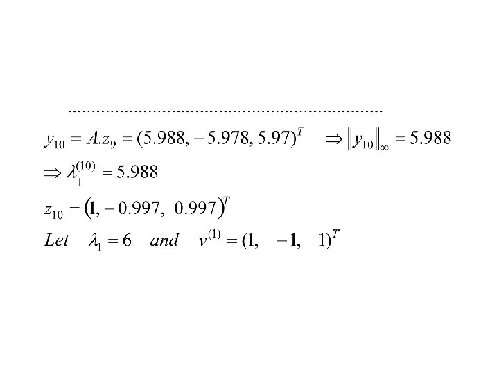
Power Method

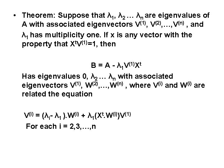
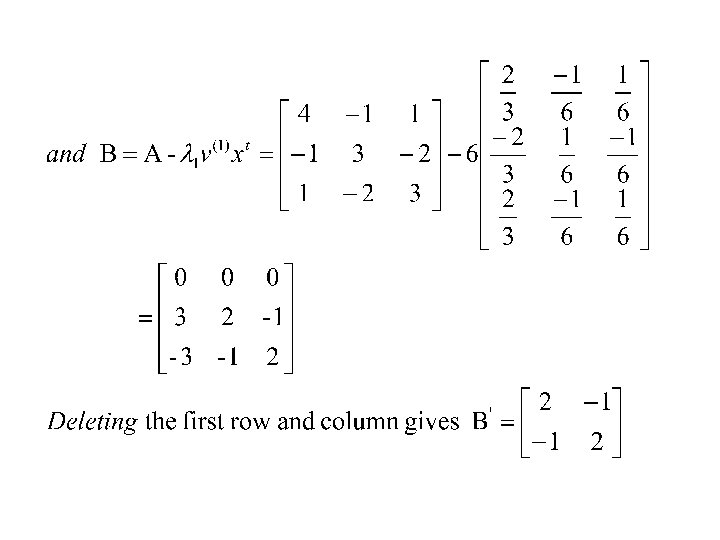
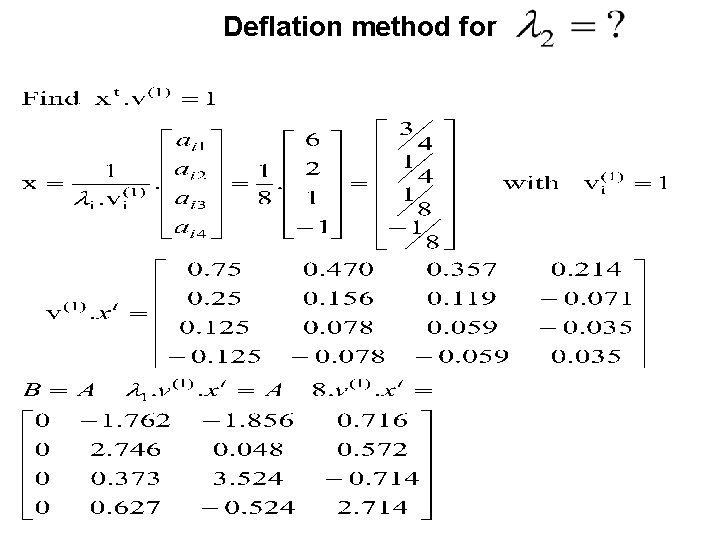
• Theorem: Suppose that λ 1, λ 2 … λn are eigenvalues of A with associated eigenvectors V(1), V(2), …, V(n) , and λ 1 has multiplicity one. If x is any vector with the property that Xt. V(1)=1, then B = A - λ 1 V(1)Xt Has eigenvalues 0, λ 2 … λn with associated eigenvectors V(1), W(2), …, W(n) , where V(i) and W(i) are related the equation V(i) = (λi- λ 1 ). W(i) + λ 1(Xt. W(i))V(1) For each i = 2, 3, …, n

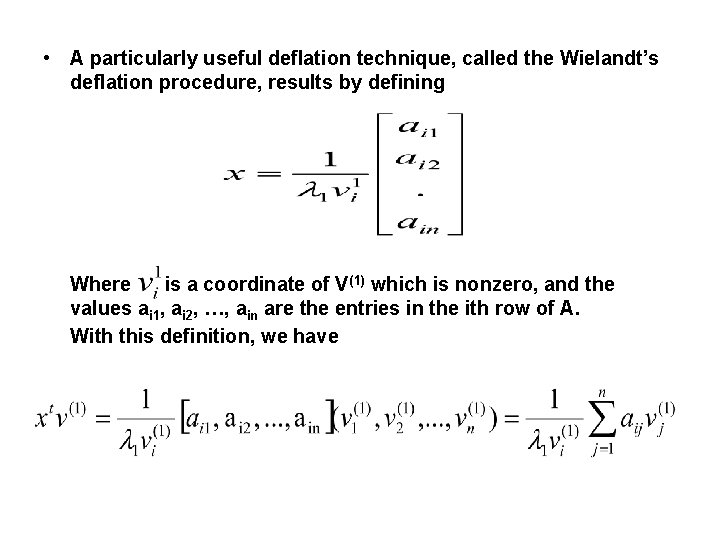
• A particularly useful deflation technique, called the Wielandt’s deflation procedure, results by defining Where is a coordinate of V(1) which is nonzero, and the values ai 1, ai 2, …, ain are the entries in the ith row of A. With this definition, we have

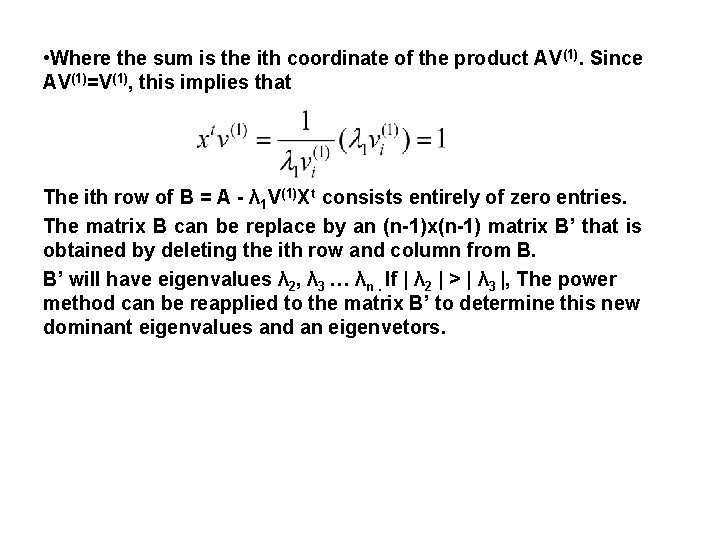
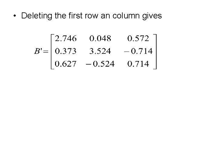
• Where the sum is the ith coordinate of the product AV(1). Since AV(1)=V(1), this implies that The ith row of B = A - λ 1 V(1)Xt consists entirely of zero entries. The matrix B can be replace by an (n-1)x(n-1) matrix B’ that is obtained by deleting the ith row and column from B. B’ will have eigenvalues λ 2, λ 3 … λn. If | λ 2 | > | λ 3 |, The power method can be reapplied to the matrix B’ to determine this new dominant eigenvalues and an eigenvetors.

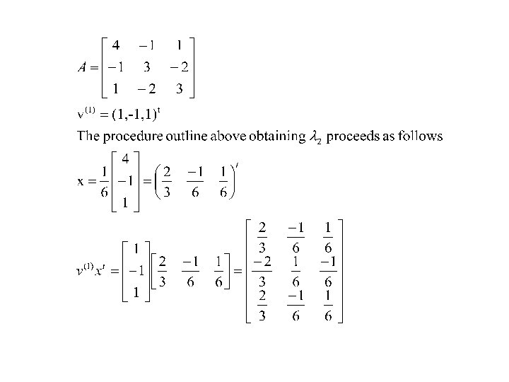
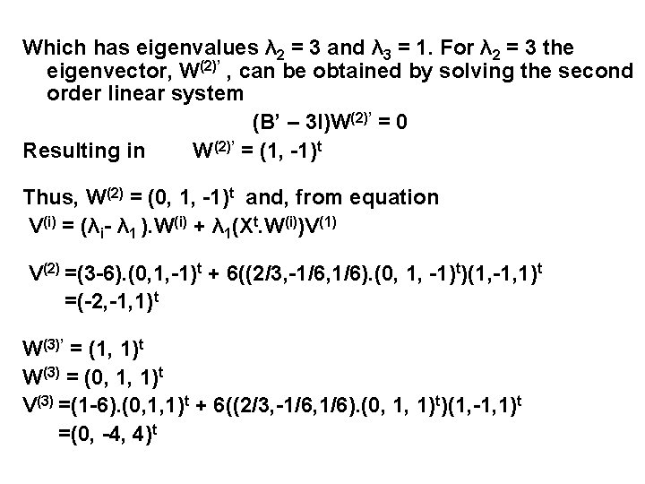
Which has eigenvalues λ 2 = 3 and λ 3 = 1. For λ 2 = 3 the eigenvector, W(2)’ , can be obtained by solving the second order linear system (B’ – 3 I)W(2)’ = 0 Resulting in W(2)’ = (1, -1)t Thus, W(2) = (0, 1, -1)t and, from equation V(i) = (λi- λ 1 ). W(i) + λ 1(Xt. W(i))V(1) V(2) =(3 -6). (0, 1, -1)t + 6((2/3, -1/6, 1/6). (0, 1, -1)t)(1, -1, 1)t =(-2, -1, 1)t W(3)’ = (1, 1)t W(3) = (0, 1, 1)t V(3) =(1 -6). (0, 1, 1)t + 6((2/3, -1/6, 1/6). (0, 1, 1)t)(1, -1, 1)t =(0, -4, 4)t

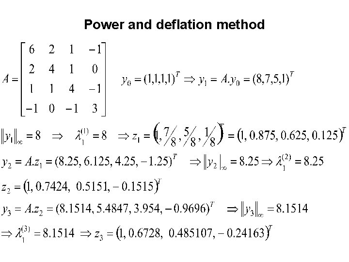
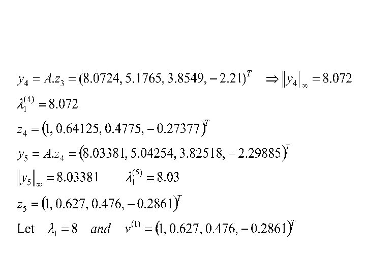
Power and deflation method

Deflation method for

• Deleting the first row an column gives