Eigen Faces and Eigen Patches Useful model of

Eigen. Faces and Eigen. Patches • Useful model of variation in a region – Region must be fixed shape (eg rectangle) • Developed for face recognition • Generalised for – face location – object location/recognition

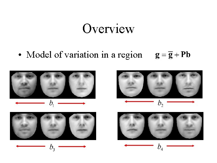
Overview • Model of variation in a region

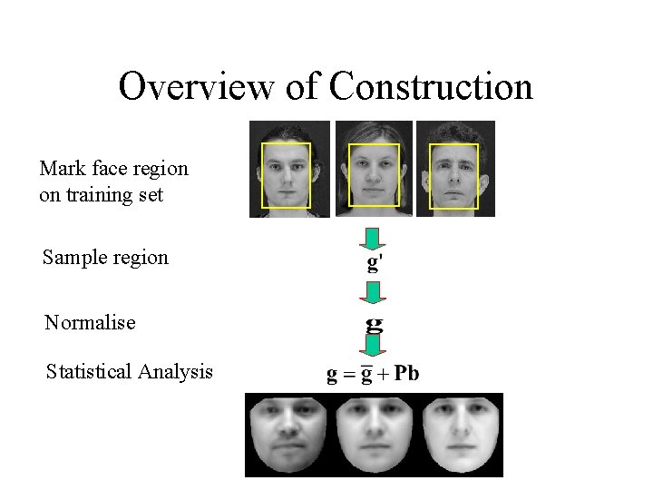
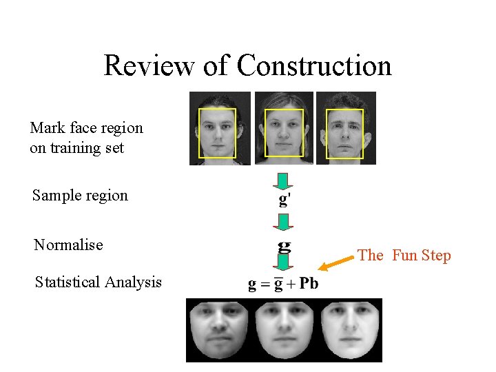
Overview of Construction Mark face region on training set Sample region Normalise Statistical Analysis

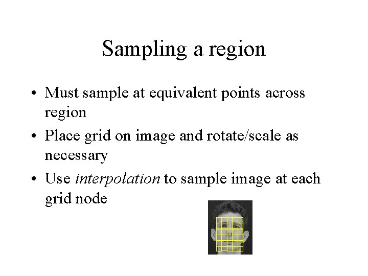
Sampling a region • Must sample at equivalent points across region • Place grid on image and rotate/scale as necessary • Use interpolation to sample image at each grid node

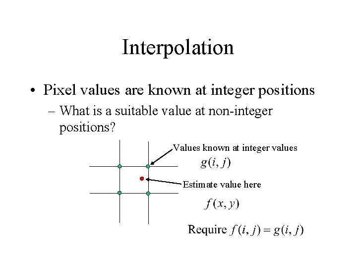
Interpolation • Pixel values are known at integer positions – What is a suitable value at non-integer positions? Values known at integer values Estimate value here

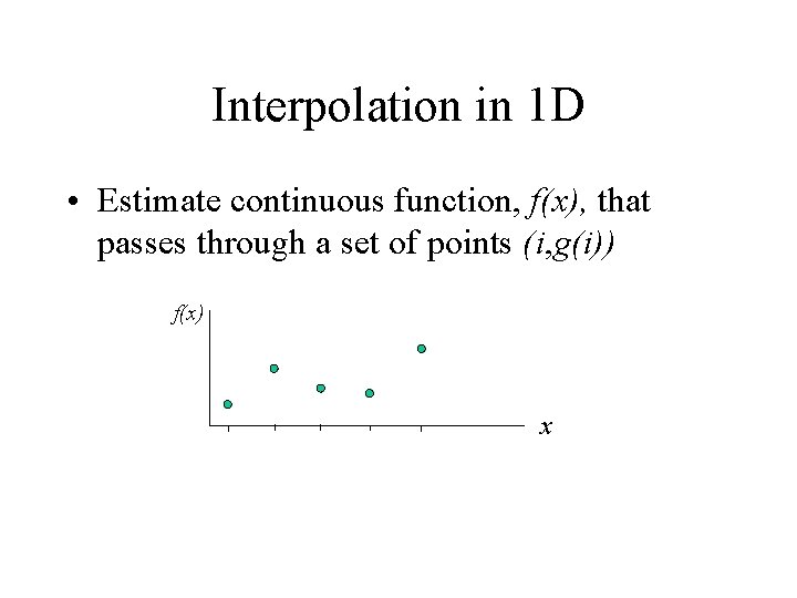
Interpolation in 1 D • Estimate continuous function, f(x), that passes through a set of points (i, g(i)) f(x) x

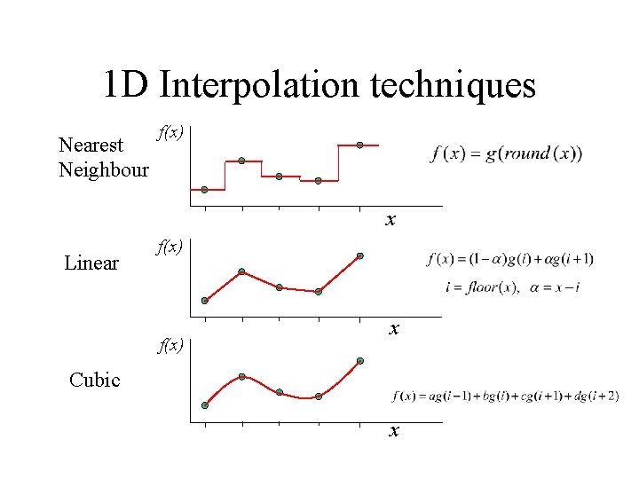
1 D Interpolation techniques Nearest Neighbour f(x) x Linear f(x) x Cubic x

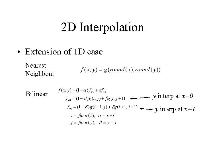
2 D Interpolation • Extension of 1 D case Nearest Neighbour Bilinear y interp at x=0 y interp at x=1

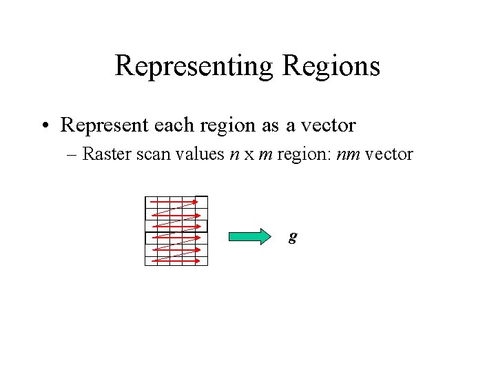
Representing Regions • Represent each region as a vector – Raster scan values n x m region: nm vector g

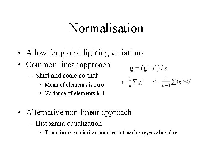
Normalisation • Allow for global lighting variations • Common linear approach – Shift and scale so that • Mean of elements is zero • Variance of elements is 1 • Alternative non-linear approach – Histogram equalization • Transforms so similar numbers of each grey-scale value

Review of Construction Mark face region on training set Sample region Normalise Statistical Analysis The Fun Step

Multivariate Statistical Analysis • Need to model the distribution of normalised vectors – Generate plausible new examples – Test if new region similar to training set – Classify region

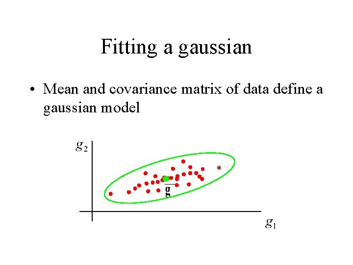
Fitting a gaussian • Mean and covariance matrix of data define a gaussian model

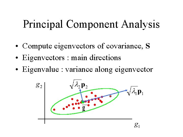
Principal Component Analysis • Compute eigenvectors of covariance, S • Eigenvectors : main directions • Eigenvalue : variance along eigenvector

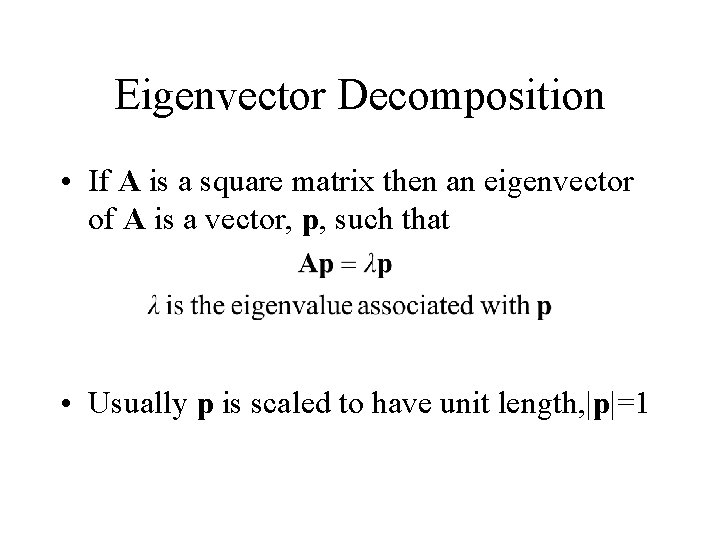
Eigenvector Decomposition • If A is a square matrix then an eigenvector of A is a vector, p, such that • Usually p is scaled to have unit length, |p|=1

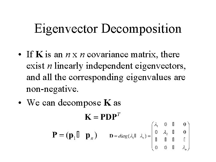
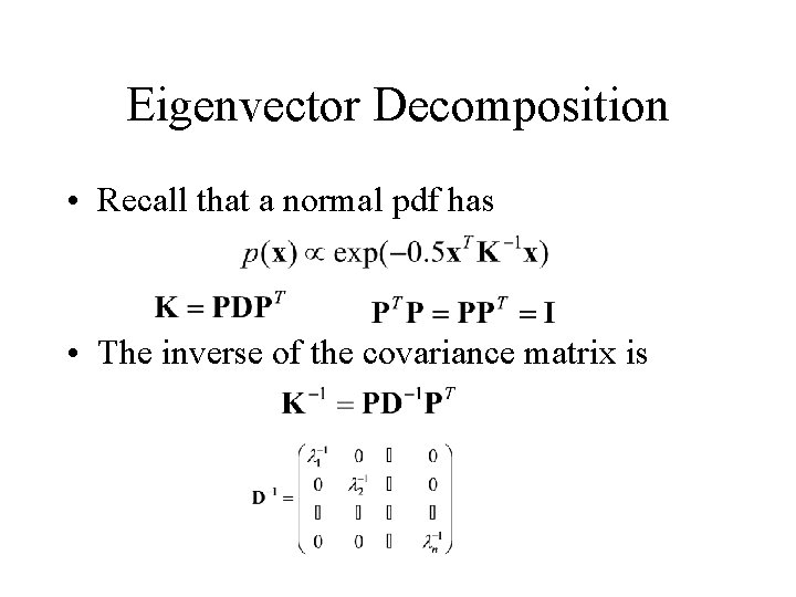
Eigenvector Decomposition • If K is an n x n covariance matrix, there exist n linearly independent eigenvectors, and all the corresponding eigenvalues are non-negative. • We can decompose K as

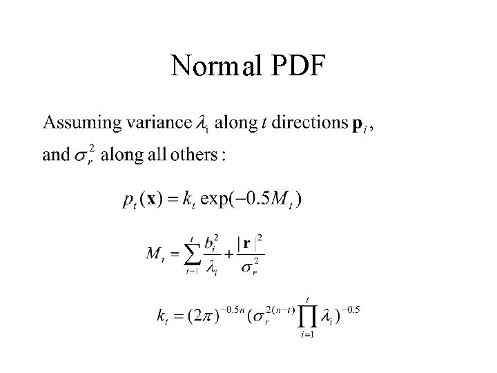
Eigenvector Decomposition • Recall that a normal pdf has • The inverse of the covariance matrix is

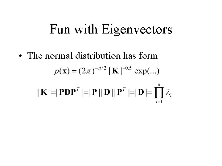
Fun with Eigenvectors • The normal distribution has form

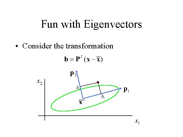
Fun with Eigenvectors • Consider the transformation

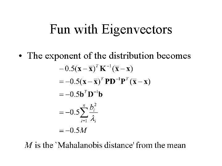
Fun with Eigenvectors • The exponent of the distribution becomes

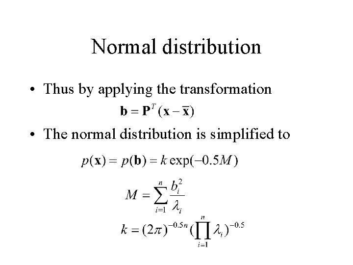
Normal distribution • Thus by applying the transformation • The normal distribution is simplified to

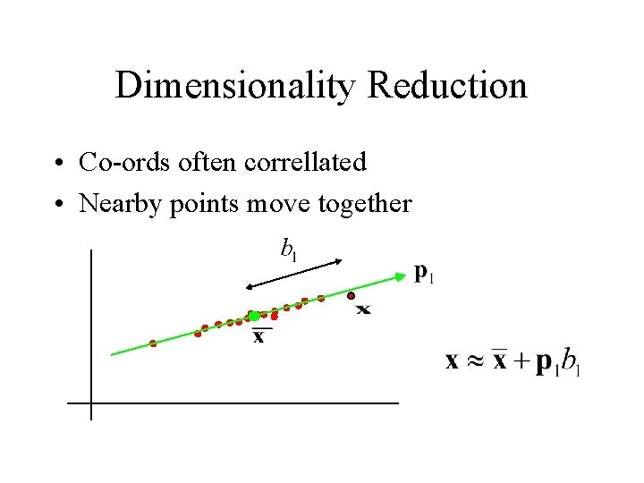
Dimensionality Reduction • Co-ords often correllated • Nearby points move together

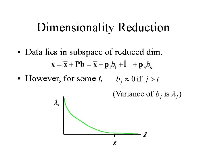
Dimensionality Reduction • Data lies in subspace of reduced dim. • However, for some t,

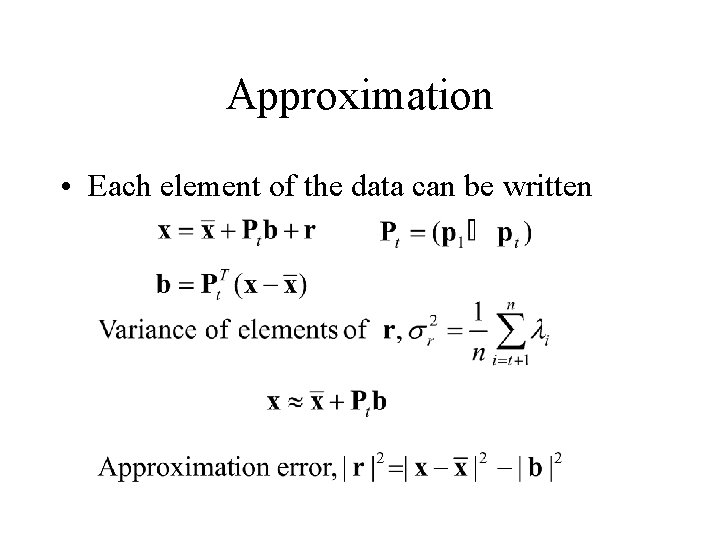
Approximation • Each element of the data can be written

Normal PDF

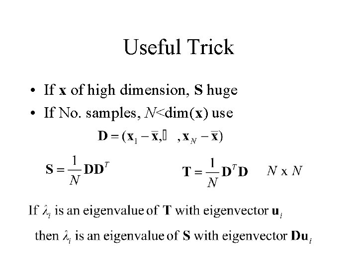
Useful Trick • If x of high dimension, S huge • If No. samples, N<dim(x) use

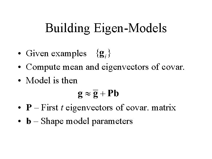
Building Eigen-Models • Given examples • Compute mean and eigenvectors of covar. • Model is then • P – First t eigenvectors of covar. matrix • b – Shape model parameters

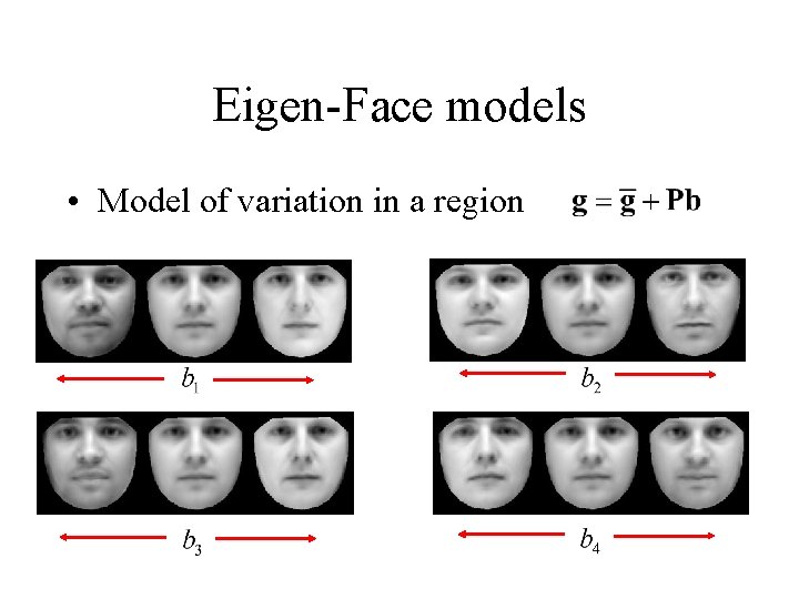
Eigen-Face models • Model of variation in a region

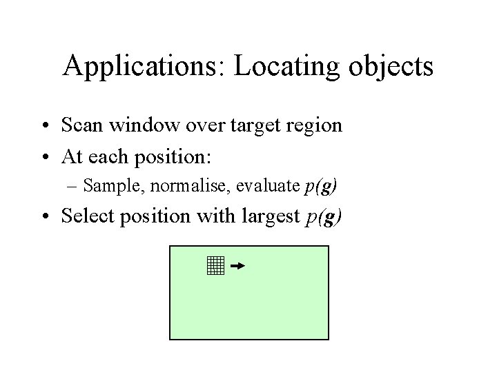
Applications: Locating objects • Scan window over target region • At each position: – Sample, normalise, evaluate p(g) • Select position with largest p(g)

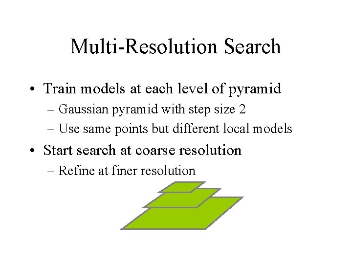
Multi-Resolution Search • Train models at each level of pyramid – Gaussian pyramid with step size 2 – Use same points but different local models • Start search at coarse resolution – Refine at finer resolution

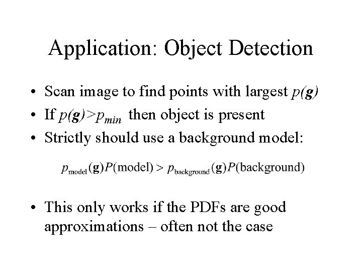
Application: Object Detection • Scan image to find points with largest p(g) • If p(g)>pmin then object is present • Strictly should use a background model: • This only works if the PDFs are good approximations – often not the case

Application: Face Recognition • Eigenfaces developed for face recognition – More about this later