Eigen Decomposition Based on the slides by Mani

Eigen Decomposition Based on the slides by Mani Thomas and book by Gilbert Strang. Modified and extended by Longin Jan Latecki

Introduction n n Eigenvalue decomposition Physical interpretation of eigenvalue/eigenvectors

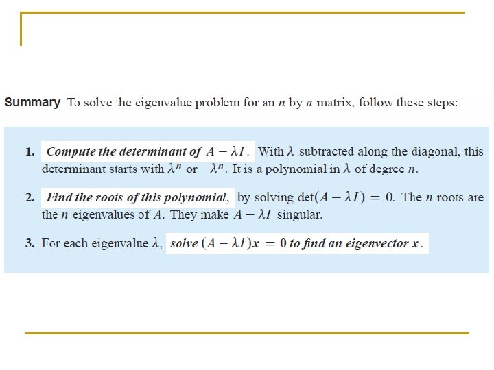
What are eigenvalues? n Given a matrix, A, x is the eigenvector and is the corresponding eigenvalue if Ax = x q A must be square and the determinant of A - I must be equal to zero Ax - x = 0 iff (A - I) x = 0 n n n Trivial solution is if x = 0 The non trivial solution occurs when det(A - I) = 0 Are eigenvectors unique? q If x is an eigenvector, then x is also an eigenvector and is an eigenvalue A( x) = (Ax) = ( x)

Calculating the Eigenvectors/values Expand the det(A - I) = 0 for a 2 x 2 matrix n n For a 2 x 2 matrix, this is a simple quadratic equation with two solutions (maybe complex) n This “characteristic equation” can be used to solve for x

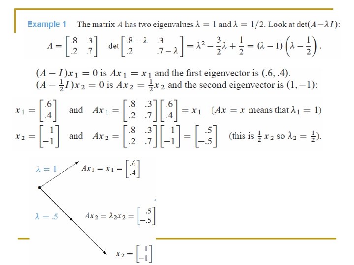
Eigenvalue example n Consider, n The corresponding eigenvectors can be computed as q q For = 0, one possible solution is x = (2, -1) For = 5, one possible solution is x = (1, 2) For more information: Demos in Linear algebra by G. Strang, http: //web. mit. edu/18. 06/www/

Eigen/diagonal Decomposition n n Let be a square matrix that has m linearly independent eigenvectors (a “nondefective” matrix) Theorem: Exists an eigen decomposition diagonal q (cf. matrix diagonalization theorem) n Columns of U are eigenvectors of S n Diagonal elements of are eigenvalues of Unique for distinct eigenvalues

Diagonal decomposition: why/how Let U have the eigenvectors as columns: Then, SU can be written Thus SU=U , or U– 1 SU= And S=U U– 1.

Diagonal decomposition example For The eigenvectors Inverting, we have Then, S=U U– 1 = and form Recall UU– 1 =1.

Example continued Let’s divide U (and multiply U– 1) by Then, S= Q Why? Stay tuned … (Q-1= QT )

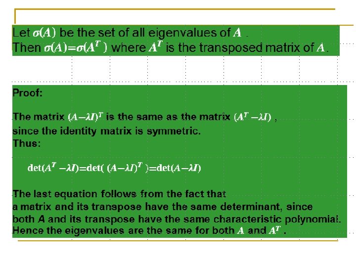
Symmetric Eigen Decomposition n If n Theorem: Exists a (unique) eigen decomposition n is a symmetric matrix: where Q is orthogonal: q Q-1= QT q Columns of Q are normalized eigenvectors q Columns are orthogonal. q (everything is real)

Physical interpretation n Consider a covariance matrix, A, i. e. , A = 1/n S ST for some S n The ellipse with the major axis as the larger eigenvalue and the minor axis as the smaller eigenvalue

Original Variable B Physical interpretation PC 2 PC 1 Original Variable A n n Orthogonal directions of greatest variance in data Projections along PC 1 (Principal Component) discriminate the data most along any one axis

Physical interpretation n n First principal component is the direction of greatest variability (covariance) in the data Second is the next orthogonal (uncorrelated) direction of greatest variability q n n So first remove all the variability along the first component, and then find the next direction of greatest variability And so on … Thus each eigenvectors provides the directions of data variances in decreasing order of eigenvalues For more information: See Gram-Schmidt Orthogonalization in G. Strang’s lectures