Efficiently Answering Reachability Queries on Large Directed Graphs

Efficiently Answering Reachability Queries on Large Directed Graphs Ruoming Jin Kent State University Joint work with Yang Xiang (KSU), Ning Ruan (KSU), and Haixun Wang (IBM T. J. Watson)

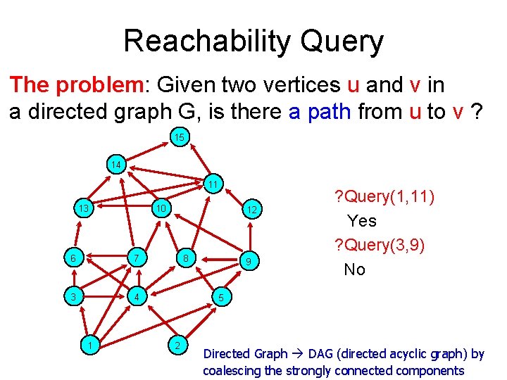
Reachability Query The problem: Given two vertices u and v in a directed graph G, is there a path from u to v ? 15 14 11 13 10 6 7 3 4 1 12 8 9 ? Query(1, 11) Yes ? Query(3, 9) No 5 2 Directed Graph DAG (directed acyclic graph) by coalescing the strongly connected components

Applications • • • XML Biological networks Graph Databases Ontology Knowledge representation (Lattice operation) Object programming (Class relationship) Distributed systems (Reachable states)

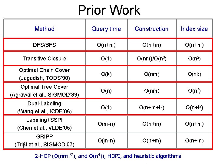
Prior Work Method Query time Construction Index size DFS/BFS O(n+m) Transitive Closure O(1) O(nm)/O(n 3) O(n 2) Optimal Chain Cover (Jagadish, TODS’ 90) O(k) O(nm) O(nk) Optimal Tree Cover (Agrawal et al. , SIGMOD’ 89) O(nm) O(n 2) Dual-Labeling (Wang et al. , ICDE’ 06) O(1) O(n+m+t 3) O(n+t 2) Labeling+SSPI (Chen et al. , VLDB’ 05) O(m-n) O(n+m) GRIPP (Triβl et al. , SIGMOD’ 07) O(m-n) O(n+m) 2 -HOP (O(nm 1/2), and O(n 4)), HOPI, and heuristic algorithms

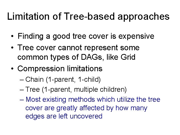
Limitation of Tree-based approaches • Finding a good tree cover is expensive • Tree cover cannot represent some common types of DAGs, like Grid • Compression limitations – Chain (1 -parent, 1 -child) – Tree (1 -parent, multiple children) – Most existing methods which utilize the tree cover are greatly affected by how many edges are left uncovered

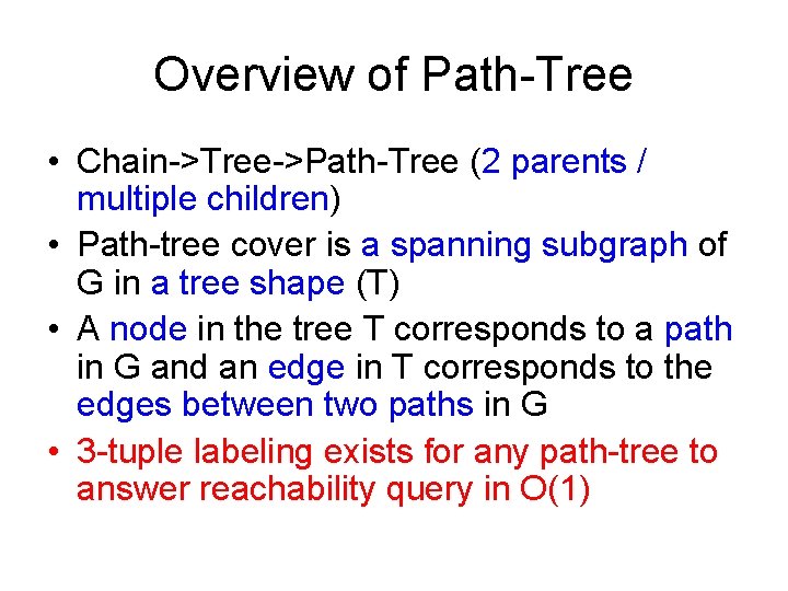
Overview of Path-Tree • Chain->Tree->Path-Tree (2 parents / multiple children) • Path-tree cover is a spanning subgraph of G in a tree shape (T) • A node in the tree T corresponds to a path in G and an edge in T corresponds to the edges between two paths in G • 3 -tuple labeling exists for any path-tree to answer reachability query in O(1)

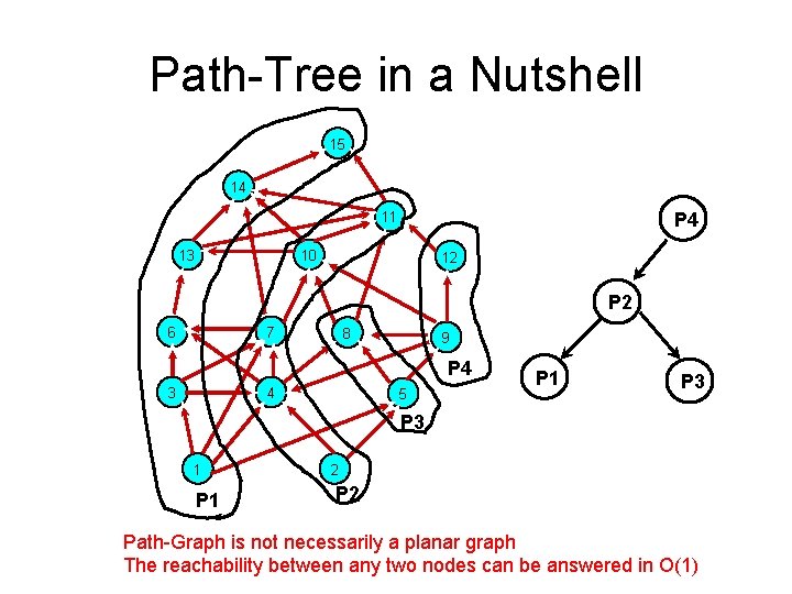
Path-Tree in a Nutshell 15 14 P 4 11 13 10 12 P 2 6 7 8 9 P 4 3 4 5 P 1 P 3 1 P 1 2 Path-Graph is not necessarily a planar graph The reachability between any two nodes can be answered in O(1)

Key Problems • How to construct a path-tree? – Algorithm • How can a path-tree help with reachability queries? – Labeling – Transitive Closure Compression • How does path-tree compare with the existing methods? – Optimality

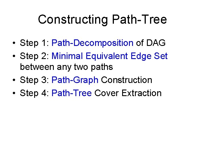
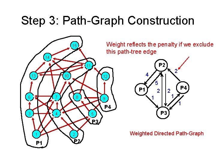
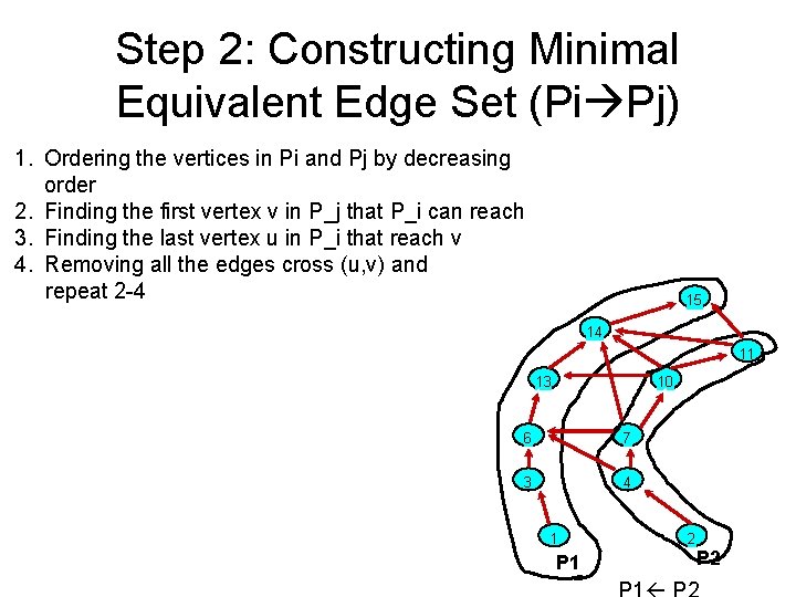
Constructing Path-Tree • Step 1: Path-Decomposition of DAG • Step 2: Minimal Equivalent Edge Set between any two paths • Step 3: Path-Graph Construction • Step 4: Path-Tree Cover Extraction

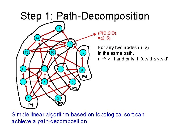
Step 1: Path-Decomposition 15 (PID, SID) =(2, 5) 14 11 13 10 6 12 7 8 For any two nodes (u, v) in the same path, u v if and only if (u. sid v. sid) 9 P 4 3 4 5 P 3 1 P 1 2 P 2 Simple linear algorithm based on topological sort can achieve a path-decomposition

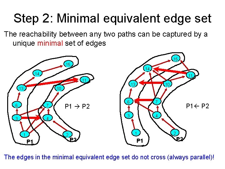
Step 2: Minimal equivalent edge set The reachability between any two paths can be captured by a unique minimal set of edges 15 15 14 14 11 11 13 13 10 6 7 3 4 1 P 1 P 2 2 P 1 10 6 7 3 4 1 P 2 P 1 P 2 2 P 2 The edges in the minimal equivalent edge set do not cross (always parallel)!

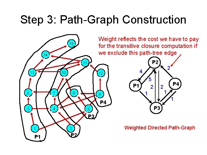
Step 3: Path-Graph Construction Weight reflects the cost we have to pay for the transitive closure computation if we exclude this path-tree edge 15 14 P 2 11 13 10 2 4 12 5 2 P 1 6 7 8 9 2 1 4 5 1 1 P 4 3 P 4 P 3 1 P 1 2 P 2 Weighted Directed Path-Graph

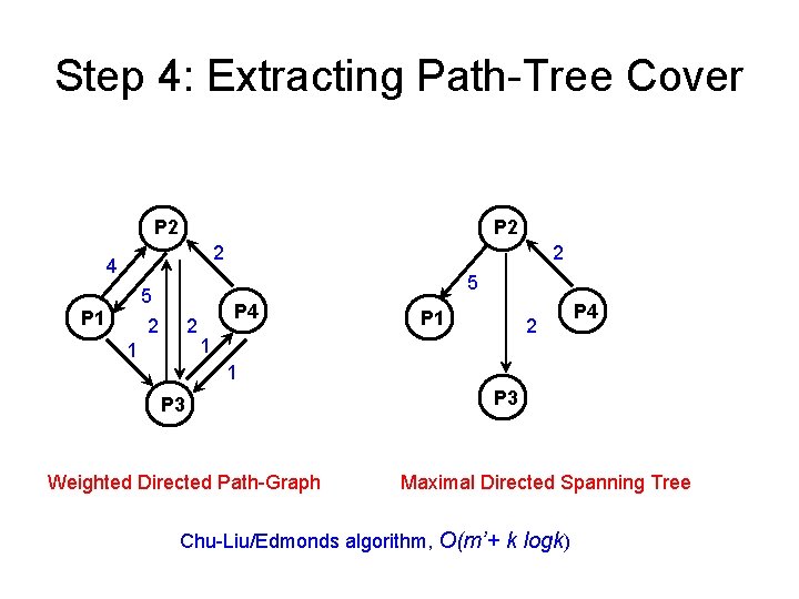
Step 4: Extracting Path-Tree Cover P 2 2 4 5 5 2 P 1 2 2 1 P 4 P 1 2 1 P 4 1 P 3 Weighted Directed Path-Graph P 3 Maximal Directed Spanning Tree Chu-Liu/Edmonds algorithm, O(m’+ k logk)

Key Problems • How to construct a path-tree? – Algorithm • How can path-tree help with reachability queries? – Labeling – Transitive Closure Compression • How does path-tree compare with the existing methods? – Optimality

3 -Tuple Labeling for Reachability P 2 15 [1, 3] 14 11 P 4 P 1 [1, 4] 13 10 12 [1, 1] P 3 [2, 2] 6 7 8 9 P 4 3 Interval labeling (2 -tuple) High-level description about paths Pi Pj ? 4 5 P 3 1 2 P 1 P 2 DFS labeling (1 -tuple)

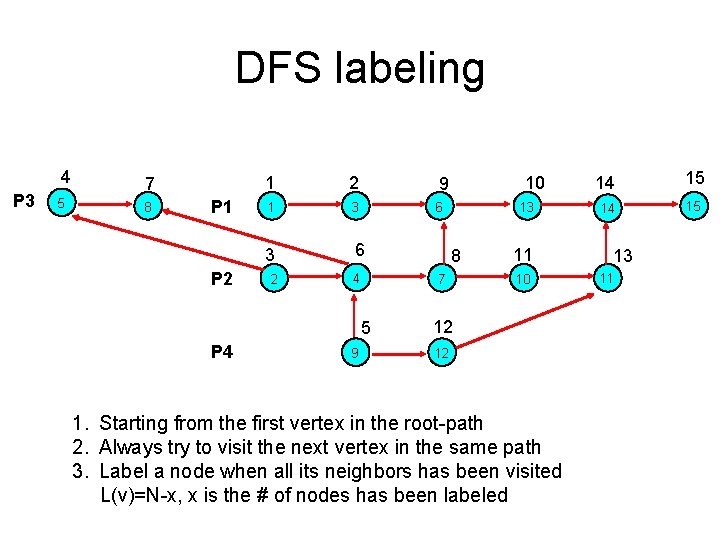
DFS labeling 4 P 3 5 7 8 P 1 P 2 1 2 9 1 3 6 2 4 9 13 8 7 5 P 4 10 11 10 12 12 1. Starting from the first vertex in the root-path 2. Always try to visit the next vertex in the same path 3. Label a node when all its neighbors has been visited L(v)=N-x, x is the # of nodes has been labeled 14 15 13 11

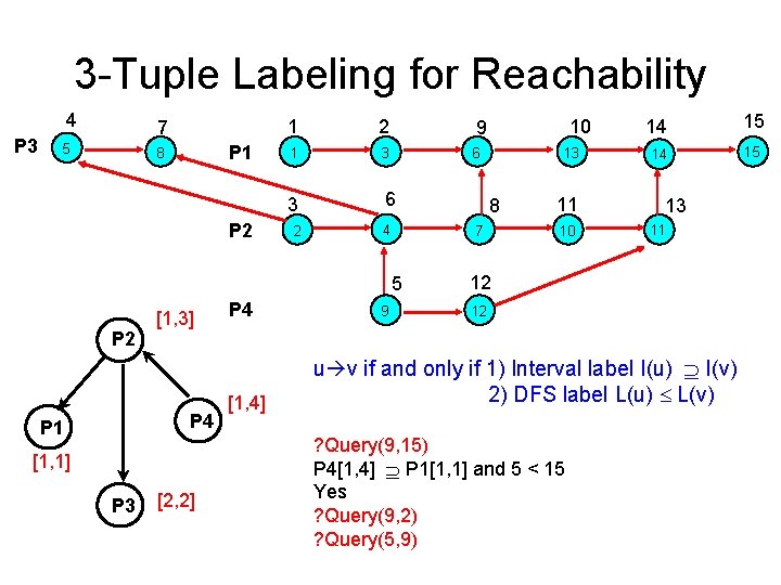
3 -Tuple Labeling for Reachability 4 P 3 7 5 P 1 8 P 2 1 2 9 1 3 6 2 4 P 2 P 4 P 1 [1, 1] P 3 [2, 2] P 4 [1, 4] 9 13 8 7 5 [1, 3] 10 11 10 14 15 13 11 12 12 u v if and only if 1) Interval label I(u) I(v) 2) DFS label L(u) L(v) ? Query(9, 15) P 4[1, 4] P 1[1, 1] and 5 < 15 Yes ? Query(9, 2) ? Query(5, 9)

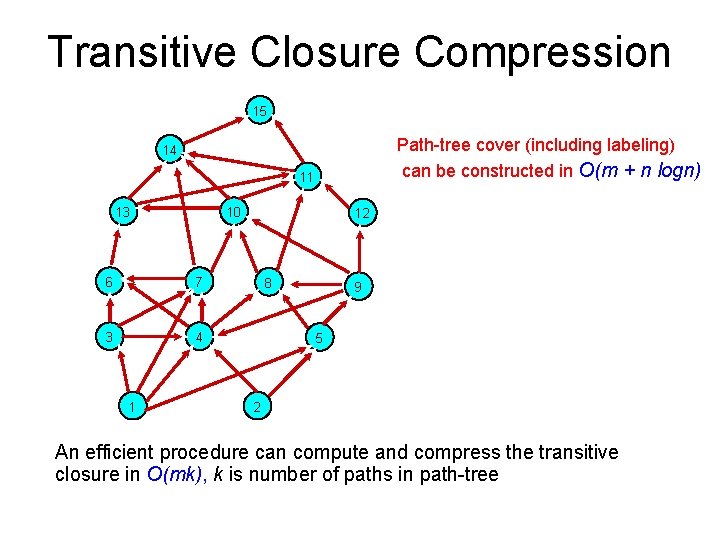
Transitive Closure Compression 15 Path-tree cover (including labeling) can be constructed in O(m + n logn) 14 11 13 10 6 7 3 4 1 12 8 9 5 2 An efficient procedure can compute and compress the transitive closure in O(mk), k is number of paths in path-tree

Key Problems • How to construct a path-tree? – Algorithm • How can path-tree help with reachability query? – Labeling – Transitive Closure Compression • How does path-tree compare with the existing methods? – Optimality

Theoretical Analysis • Optimal Path-Tree Cover (OPTC) Problem: – Given a path-decomposition, what is the optimal pathtree cover to maximally compress the transitive closure? – Opt. Index weight assignment based on computing the predecessor set • Optimal Path-Decomposition (OPD) Problem: – Assuming we only use path-decomposition to compress the transitive closure, what is the optimal path-decomposition to maximally compress the transitive closure? – Minimal-cost flow problem – What is the overall optimal path-decomposition?

Superiority of Path-Tree Cover • The optimal tree cover is a special case of path-tree cover when each vertex corresponds to a single path and the weight is based on Opt. Index. • The path-tree cover approach can compress the transitive closure with size being smaller than or equal to the optimal tree cover approach (and consequently optimal chain cover approach).

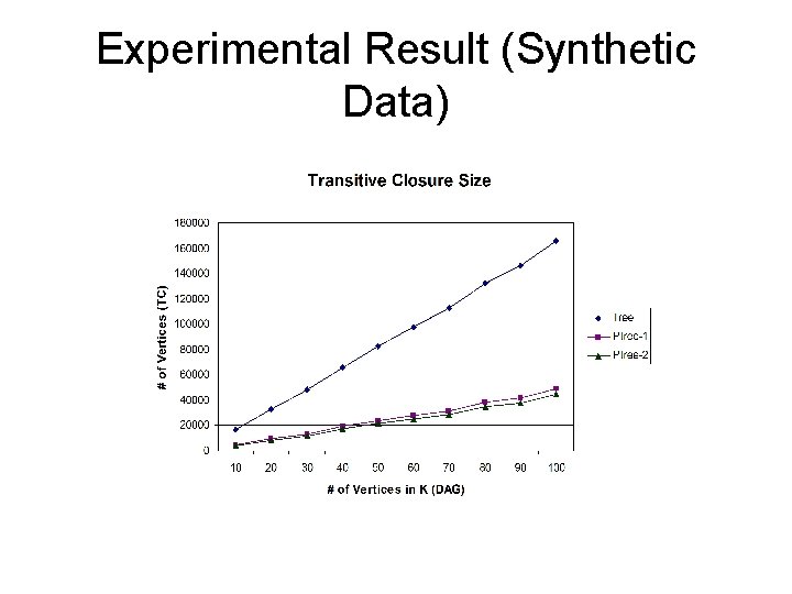
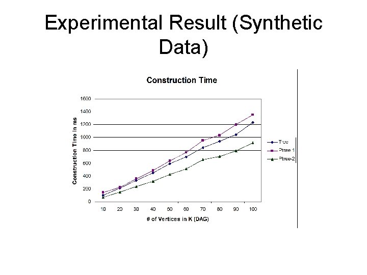
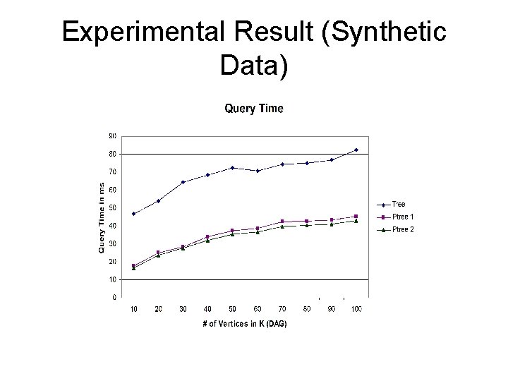
Experimental Evaluation • Implementation in C++ • 12 Real datasets used in Dual-labeling paper and GRIPP paper • Synthetic datasets – Sparse DAG with edge density = 2 • AMD Opteron 2. 0 GHz/ 2 GB/ Linux • PTree 1 (Opt. Index) and PTree 2 – Mainly compare with Optimal Tree Cover

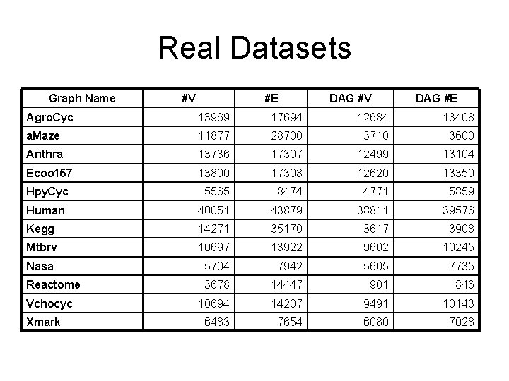
Real Datasets Graph Name #V #E DAG #V DAG #E Agro. Cyc 13969 17694 12684 13408 a. Maze 11877 28700 3710 3600 Anthra 13736 17307 12499 13104 Ecoo 157 13800 17308 12620 13350 Hpy. Cyc 5565 8474 4771 5859 Human 40051 43879 38811 39576 Kegg 14271 35170 3617 3908 Mtbrv 10697 13922 9602 10245 Nasa 5704 7942 5605 7735 Reactome 3678 14447 901 846 10694 14207 9491 10143 6483 7654 6080 7028 Vchocyc Xmark

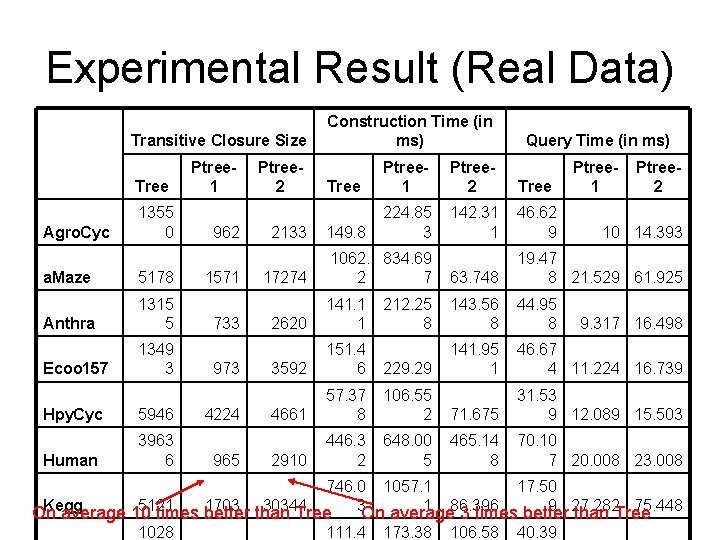
Experimental Result (Real Data) Transitive Closure Size Construction Time (in ms) Query Time (in ms) Ptree 1 Tree Ptree 1 Ptree 2 Tree Ptree 1 149. 8 224. 85 3 142. 31 1 46. 62 9 1062. 834. 69 2 7 63. 748 19. 47 8 21. 529 61. 925 2620 141. 1 1 212. 25 8 143. 56 8 44. 95 8 3592 151. 4 6 229. 29 141. 95 1 46. 67 4 11. 224 16. 739 4661 57. 37 8 106. 55 2 71. 675 31. 53 9 12. 089 15. 503 2910 446. 3 2 648. 00 5 465. 14 8 70. 10 7 20. 008 23. 008 Tree Agro. Cyc 1355 0 a. Maze 5178 Anthra 1315 5 Ecoo 157 1349 3 Hpy. Cyc 5946 Human 3963 6 962 1571 733 973 4224 965 Ptree 2 2133 17274 Ptree 2 10 14. 393 9. 317 16. 498 746. 0 1057. 1 17. 50 Kegg 5121 1703 than 30344 1 86. 396 9 27. 282 75. 448 On average 10 times better Tree 3 On average 3 times better than Tree 1028 111. 4 173. 38 106. 58 40. 39

Experimental Result (Synthetic Data)

Experimental Result (Synthetic Data)

Experimental Result (Synthetic Data)

Conclusion • A novel Path-Tree structure is proposed to assist the compression of transitive closure and answering reachability query • Path-tree has potential to integrate with other existing methods to further improve the efficiency of reachability query processing

Thanks!!

Step 3: Path-Graph Construction Weight reflects the penalty if we exclude this path-tree edge 15 14 P 2 11 13 10 2 4 12 5 2 P 1 6 7 8 9 2 1 4 5 1 1 P 4 3 P 4 P 3 1 P 1 2 P 2 Weighted Directed Path-Graph

Step 2: Constructing Minimal Equivalent Edge Set (Pi Pj) 1. Ordering the vertices in Pi and Pj by decreasing order 2. Finding the first vertex v in P_j that P_i can reach 3. Finding the last vertex u in P_i that reach v 4. Removing all the edges cross (u, v) and repeat 2 -4 15 14 11 13 10 6 7 3 4 1 P 1 2 P 2

3 -Tuple Labeling for Reachability P 2 15 [1, 3] 14 11 P 4 P 1 [1, 4] 13 10 12 [1, 1] P 3 [2, 2] 6 7 8 9 P 4 3 Interval labeling (2 -tuple) High-level description about paths Pi Pj ? 4 5 P 3 1 2 P 1 P 2 DFS labeling (1 -tuple)