Efficient Influence Maximization in Largescale Social Networks Chuan

计算社会科学与社会计算前沿研讨会 Efficient Influence Maximization in Large-scale Social Networks Chuan Zhou (周川) Institute of Information Engineering, CAS August 27, 2016

Contents 4 Network Coarsening Method 1 Introduction Efficient Influence Maximization in Large-scale Social Networks 3 Subgraph Stream Method 2 Upper Bound Method

Contents 4 Network Coarsening Method 1 Introduction Efficient Influence Maximization in Large-scale Social Networks 3 Subgraph Stream Method 2 Upper Bound Method

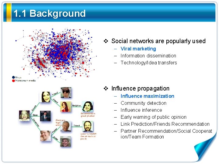
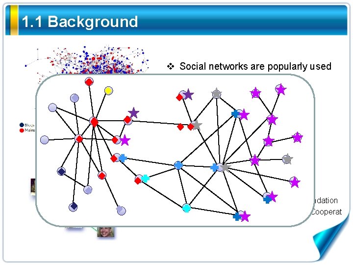
1. 1 Background v Social networks are popularly used – Viral marketing – Information dissemination – Technology/Idea transfers v Influence propagation – – – Influence maximization Community detection Influence inference Early warning of public opinion Link Prediction/Friends Recommendation Partner Recommendation/Social Cooperat ion/Team Formation

1. 1 Background v Social networks are popularly used – Viral marketing – Information dissemination – Technology/Idea transfers v Influence propagation – – – Influence maximization Community detection Influence inference Early warning of public opinion Link Prediction/Friends Recommendation Partner Recommendation/Social Cooperat ion/Team Formation

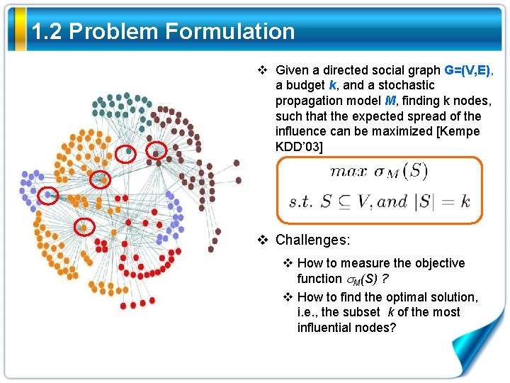
1. 2 Problem Formulation v Given a directed social graph G=(V, E), a budget k, and a stochastic propagation model M, finding k nodes, such that the expected spread of the influence can be maximized [Kempe KDD’ 03] v Challenges: v How to measure the objective function M(S) ? v How to find the optimal solution, i. e. , the subset k of the most influential nodes?

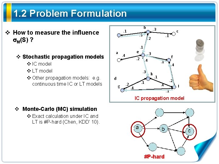
1. 2 Problem Formulation v How to measure the influence M(S) ? v Stochastic propagation models v IC model v LT model v Other propagation models: e. g. continuous time IC or LT models b . 1 a . 3 e . 4 . 1. 3. 4. 3 g . 2 . 1. 4 c . 1 . 2 d . 3 f . 1 h . 4 . 1 . 2 . 4. 1 I IC propagation model v Monte-Carlo (MC) simulation v Exact calculation under IC and LT is #P-hard (Chen, KDD’ 10). #P-hard

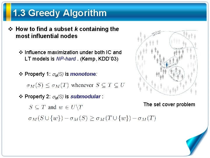
1. 3 Greedy Algorithm v How to find a subset k containing the most influential nodes v Influence maximization under both IC and LT models is NP-hard. (Kemp, KDD’ 03) v Property 1: M(S) is monotone: v Property 2: M(S) is submodular : The set cover problem

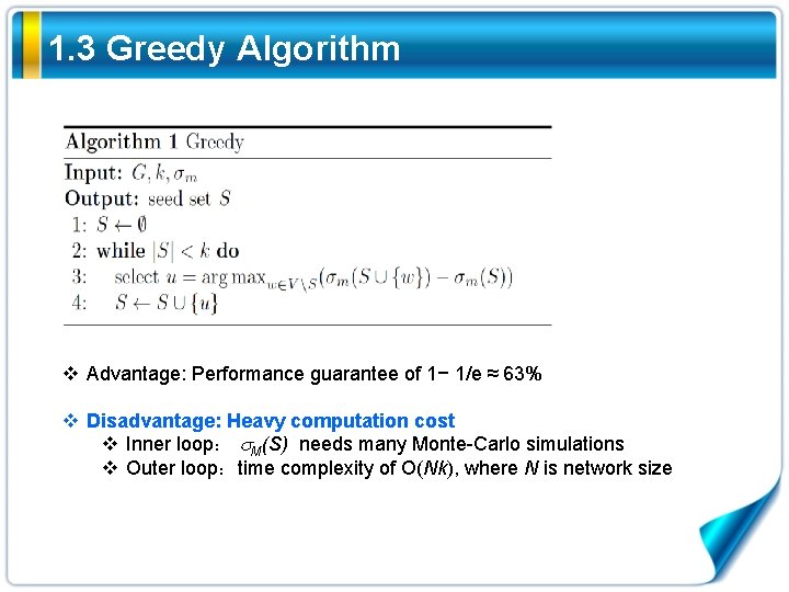
1. 3 Greedy Algorithm v Advantage: Performance guarantee of 1− 1/e ≈ 63% v Disadvantage: Heavy computation cost v Inner loop： M(S) needs many Monte-Carlo simulations v Outer loop：time complexity of O(Nk), where N is network size

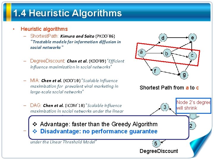
1. 4 Heuristic Algorithms • Heuristic algorithms – Shortest. Path: Kimura and Saito (PKDD’ 06) “Tractable models for information diffusion in social networks” – Degree. Discount: Chen et al. (KDD'09) “Efficient influence maximization in social networks” – MIA: Chen et al. (KDD'10) “Scalable influence maximization for prevalent viral marketing in large-scale social networks” e d f g Shortest Path from a to c Node 2’s degree will shrink – DAG: Chen et al. (ICDM’ 10) “Scalable influence maximization in social networks under the linear threshold model” v Advantage: faster than the Greedy Algorithm – SIMPATH： Goyal et al. (ICDM’ 11)“SIMPATH: v Disadvantage: no performance guarantee An Efficient Algorithm for Influence Maximization under the Linear Threshold Model” 5 Degree. Discount 2

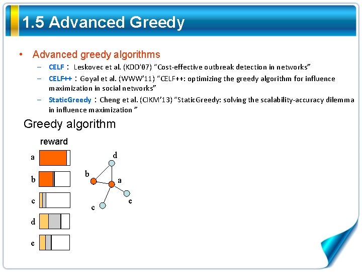
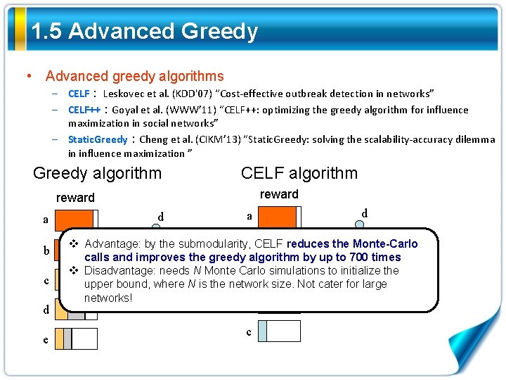
1. 5 Advanced Greedy • Advanced greedy algorithms – CELF： Leskovec et al. (KDD'07) “Cost-effective outbreak detection in networks” – CELF++：Goyal et al. (WWW’ 11) “CELF++: optimizing the greedy algorithm for influence maximization in social networks” – Static. Greedy：Cheng et al. (CIKM’ 13) “Static. Greedy: solving the scalability-accuracy dilemma in influence maximization ” Greedy algorithm reward d a b c d e b a c e

1. 5 Advanced Greedy • Advanced greedy algorithms – CELF： Leskovec et al. (KDD'07) “Cost-effective outbreak detection in networks” – CELF++：Goyal et al. (WWW’ 11) “CELF++: optimizing the greedy algorithm for influence maximization in social networks” – Static. Greedy：Cheng et al. (CIKM’ 13) “Static. Greedy: solving the scalability-accuracy dilemma in influence maximization ” Greedy algorithm reward d a b c d e b a c e

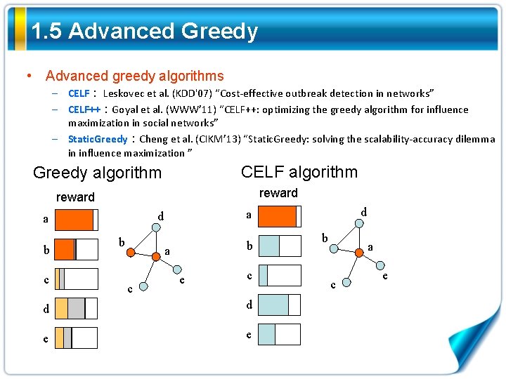
1. 5 Advanced Greedy • Advanced greedy algorithms – CELF： Leskovec et al. (KDD'07) “Cost-effective outbreak detection in networks” – CELF++：Goyal et al. (WWW’ 11) “CELF++: optimizing the greedy algorithm for influence maximization in social networks” – Static. Greedy：Cheng et al. (CIKM’ 13) “Static. Greedy: solving the scalability-accuracy dilemma in influence maximization ” CELF algorithm Greedy algorithm reward b c b b a c d a e c d d e e b a c e

1. 5 Advanced Greedy • Advanced greedy algorithms – CELF： Leskovec et al. (KDD'07) “Cost-effective outbreak detection in networks” – CELF++：Goyal et al. (WWW’ 11) “CELF++: optimizing the greedy algorithm for influence maximization in social networks” – Static. Greedy：Cheng et al. (CIKM’ 13) “Static. Greedy: solving the scalability-accuracy dilemma in influence maximization ” Greedy algorithm CELF algorithm reward b c b b a c d a e c d d e e b a c e

1. 5 Advanced Greedy • Advanced greedy algorithms – CELF： Leskovec et al. (KDD'07) “Cost-effective outbreak detection in networks” – CELF++：Goyal et al. (WWW’ 11) “CELF++: optimizing the greedy algorithm for influence maximization in social networks” – Static. Greedy：Cheng et al. (CIKM’ 13) “Static. Greedy: solving the scalability-accuracy dilemma in influence maximization ” Greedy algorithm CELF algorithm reward a b c d e d a d b the Monte-Carlo b v Advantage: by the submodularity, CELF reduces d a the greedy algorithm by up to 700 atimes calls and improves v Disadvantage: needs N Monte Carlo simulations to initialize the b e e upper bound, where N is the network size. Not cater for large c c networks! e c

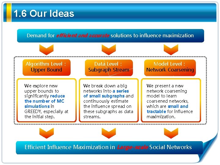
1. 6 Our Ideas Demand for efficient and accurate solutions to influence maximization Algorithm Level： Upper Bound Data Level： Subgraph Stream Model Level： Network Coarsening We explore new upper bounds to significantly reduce the number of MC simulations in GREEDY, especially at the initial step. We break down a big networks into a series of small subgraphs and continuously estimate the influence spread on these subgraphs as data streams. We present a new network coarsening model to learn coarsened networks, which are small and tractable for influence maximization. Efficient Influence Maximization in Large-scale Social Networks

Contents 4 Network Coarsening Method 1 Introduction Efficient Influence Maximization in Large-scale Social Networks 3 Subgraph Stream Method 2 Upper Bound Method

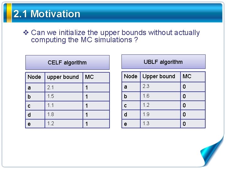
2. 1 Motivation v Can we initialize the upper bounds without actually computing the MC simulations ? UBLF algorithm CELF algorithm Node upper bound MC Node Upper bound MC a 2. 1 1 a 2. 3 0 b 1. 5 1 b 1. 6 0 c 1. 1 1 c 1. 2 0 d 1. 8 1 d 1. 9 0 e 1. 2 1 e 1. 3 0

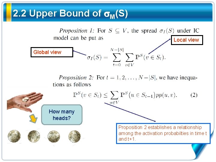
2. 2 Upper Bound of M(S) Local view Global view How many heads? Proposition 2 establishes a relationship among the activation probabilties in time t and t+1.

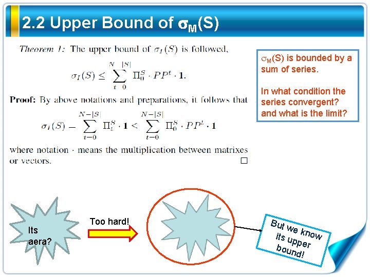
2. 2 Upper Bound of M(S) is bounded by a sum of series. In what condition the series convergent? and what is the limit? Its aera? Too hard! But w e its u know pper boun d!

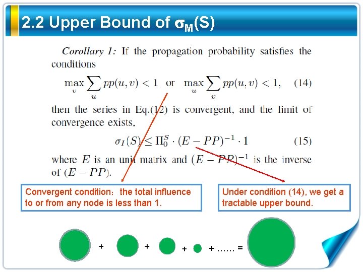
2. 2 Upper Bound of M(S) Convergent condition：the total influence to or from any node is less than 1. Under condition (14), we get a tractable upper bound. + …… =

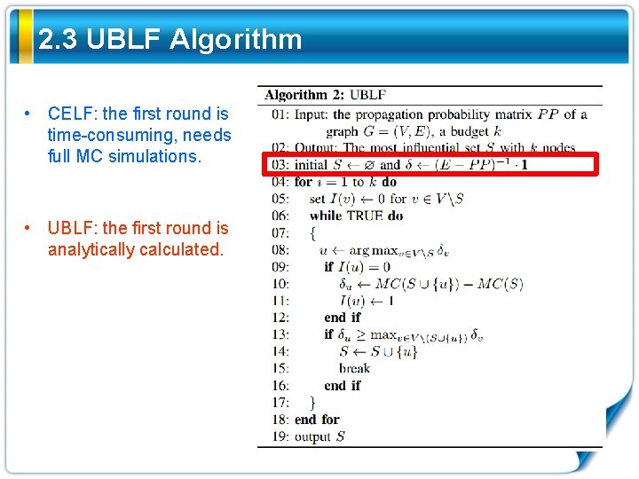
2. 3 UBLF Algorithm • CELF: the first round is time-consuming, needs full MC simulations. • UBLF: the first round is analytically calculated.

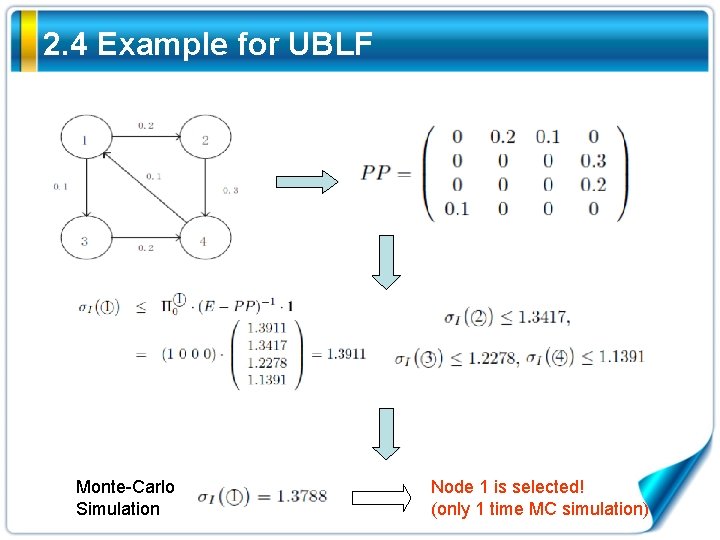
2. 4 Example for UBLF Monte-Carlo Simulation Node 1 is selected! (only 1 time MC simulation)

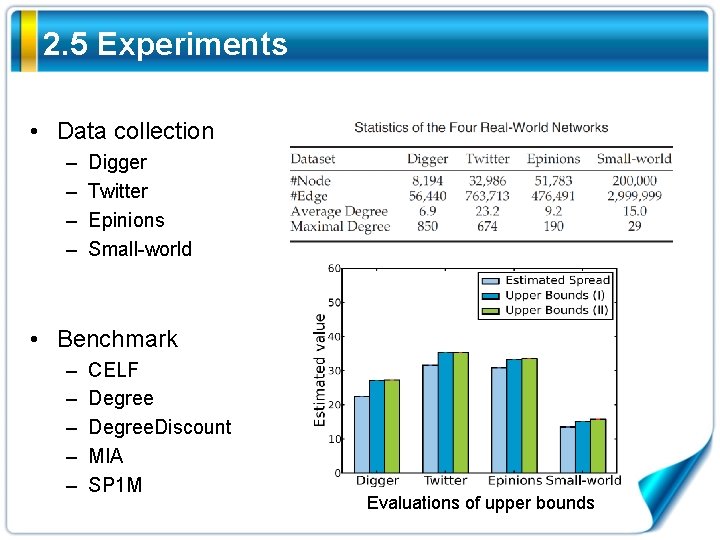
2. 5 Experiments • Data collection – – Digger Twitter Epinions Small-world • Benchmark – – – CELF Degree. Discount MIA SP 1 M Evaluations of upper bounds

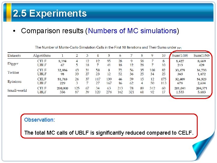
2. 5 Experiments • Comparison results (Numbers of MC simulations) Observation: The total MC calls of UBLF is significantly reduced compared to CELF.

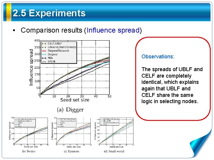
2. 5 Experiments • Comparison results (Influence spread) Observations: The spreads of UBLF and CELF are completely identical, which explains again that UBLF and CELF share the same logic in selecting nodes.

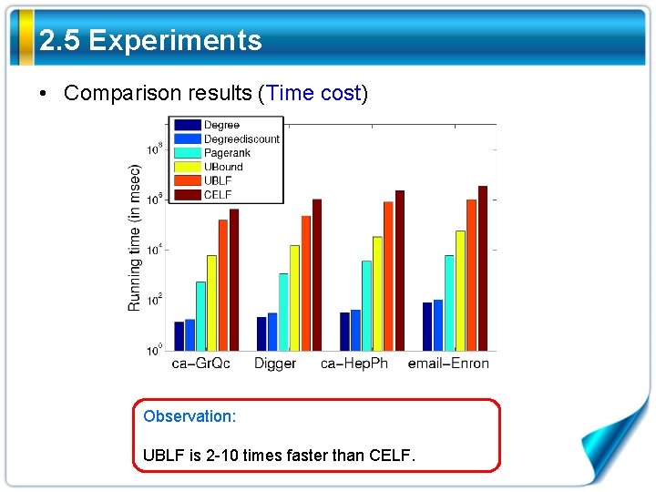
2. 5 Experiments • Comparison results (Time cost) Observation: UBLF is 2 -10 times faster than CELF.

Contents 4 Network Coarsening Method 1 Introduction Efficient Influence Maximization in Large-scale Social Networks 3 Subgraph Stream Method 2 Upper Bound Method

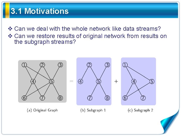
3. 1 Motivations v Can we deal with the whole network like data streams? v Can we restore results of original network from results on the subgraph streams?

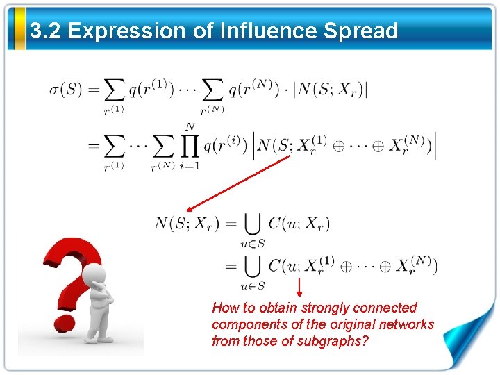
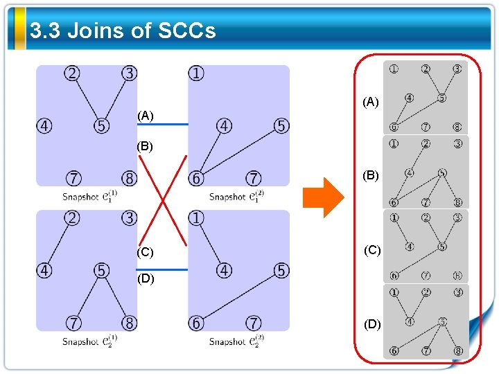
3. 2 Expression of Influence Spread How to obtain strongly connected components of the original networks from those of subgraphs?

3. 3 Joins of SCCs (A) (B) (C) (D)

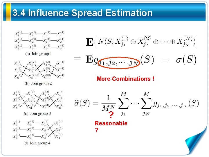
3. 4 Influence Spread Estimation More Combinations ! ? Reasonable ?

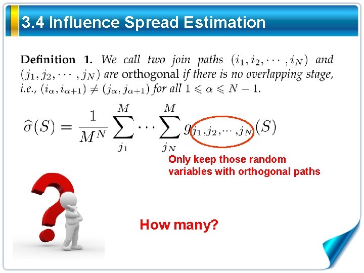
3. 4 Influence Spread Estimation Only keep those random variables with orthogonal paths How many?

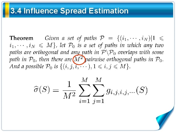
3. 4 Influence Spread Estimation

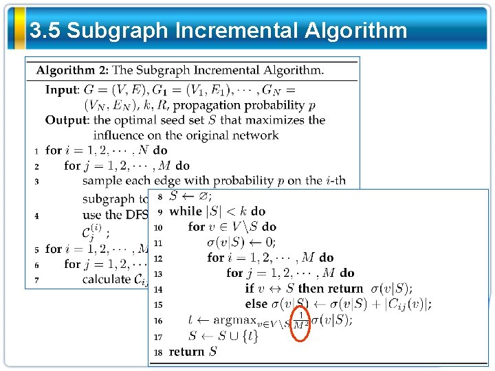
3. 5 Subgraph Incremental Algorithm

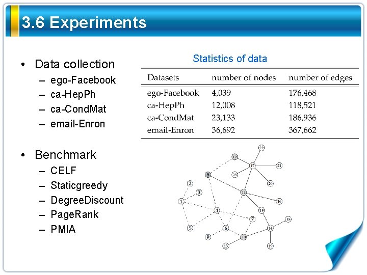
3. 6 Experiments • Data collection – – ego-Facebook ca-Hep. Ph ca-Cond. Mat email-Enron • Benchmark – – – CELF Staticgreedy Degree. Discount Page. Rank PMIA Statistics of data

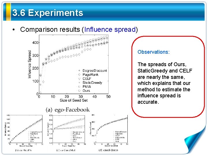
3. 6 Experiments • Comparison results (Influence spread) Observations: The spreads of Ours, Static. Greedy and CELF are nearly the same, which explains that our method to estimate the influence spread is accurate.

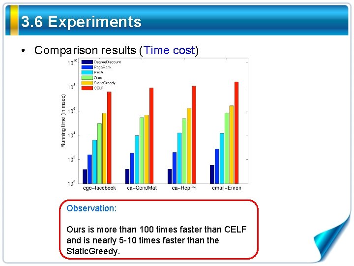
3. 6 Experiments • Comparison results (Time cost) Observation: Ours is more than 100 times faster than CELF and is nearly 5 -10 times faster than the Static. Greedy.

Contents 4 Network Coarsening Method 1 Introduction Efficient Influence Maximization in Large-scale Social Networks 3 Subgraph Stream Method 2 Upper Bound Method

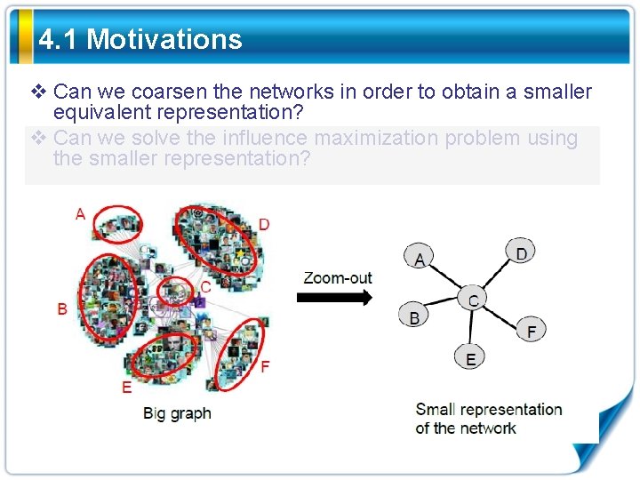
4. 1 Motivations v Can we coarsen the networks in order to obtain a smaller equivalent representation? v Can we solve the influence maximization problem using the smaller representation?

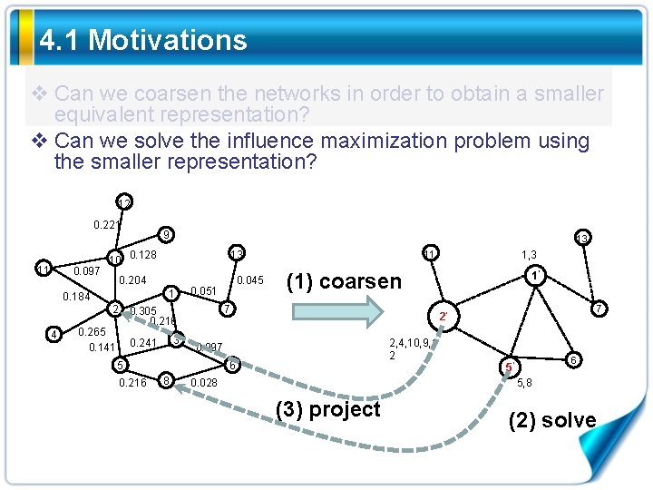
4. 1 Motivations v Can we coarsen the networks in order to obtain a smaller equivalent representation? v Can we solve the influence maximization problem using the smaller representation? 12 0. 221 11 0. 097 9 10 0. 128 1 2 3 0. 241 1’ 7 2’ 2, 4, 10, 9, 1 2 0. 097 6 8 1, 3 (1) coarsen 7 5 0. 216 0. 045 0. 051 0. 305 0. 216 0. 265 0. 141 11 13 0. 204 0. 184 4 13 0. 028 6 5’ 5, 8 (3) project (2) solve

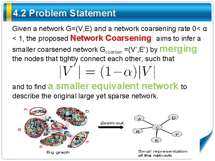
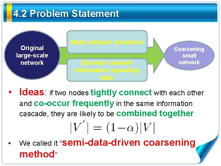
4. 2 Problem Statement Given a network G=(V, E) and a network coarsening rate 0< α < 1, the proposed Network Coarsening aims to infer a smaller coarsened network Gcoarsen =(V’, E’) by merging the nodes that tightly connect each other, such that and to find a smaller equivalent network to describe the original large yet sparse network.

4. 2 Problem Statement Original large-scale network Static network structures Dynamic network information spreading data Coarsening small network • Ideas: if two nodes tightly connect with each other and co-occur frequently in the same information cascade, they are likely to be combined together • We called it “semi-data-driven method” coarsening

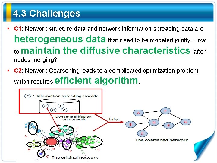
4. 3 Challenges • C 1: Network structure data and network information spreading data are heterogeneous data that need to be modeled jointly. How to maintain the diffusive characteristics after nodes merging? • C 2: Network Coarsening leads to a complicated optimization problem which requires efficient algorithm.

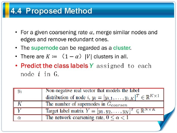
4. 4 Proposed Method

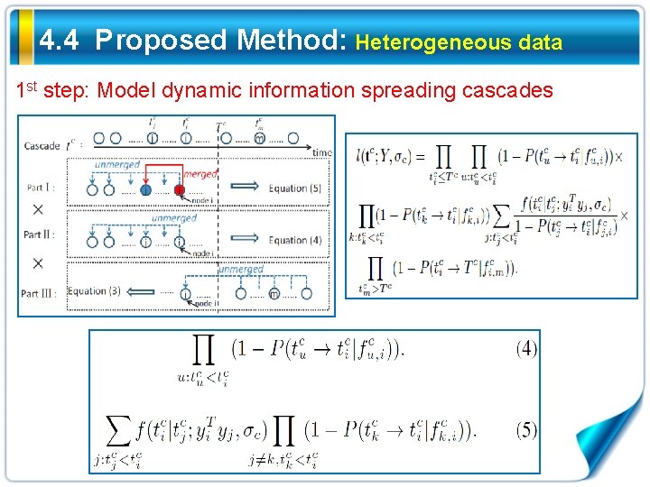
4. 4 Proposed Method: Heterogeneous data 1 st step: Model dynamic information spreading cascades

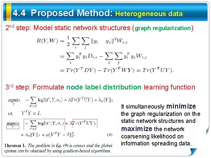
4. 4 Proposed Method: Heterogeneous data 2 nd step: Model static network structures (graph regularization) 3 rd step: Formulate node label distribution learning function It simultaneously minimize the graph regularization on the static network structures and maximize the network coarsening likelihood on information spreading data.

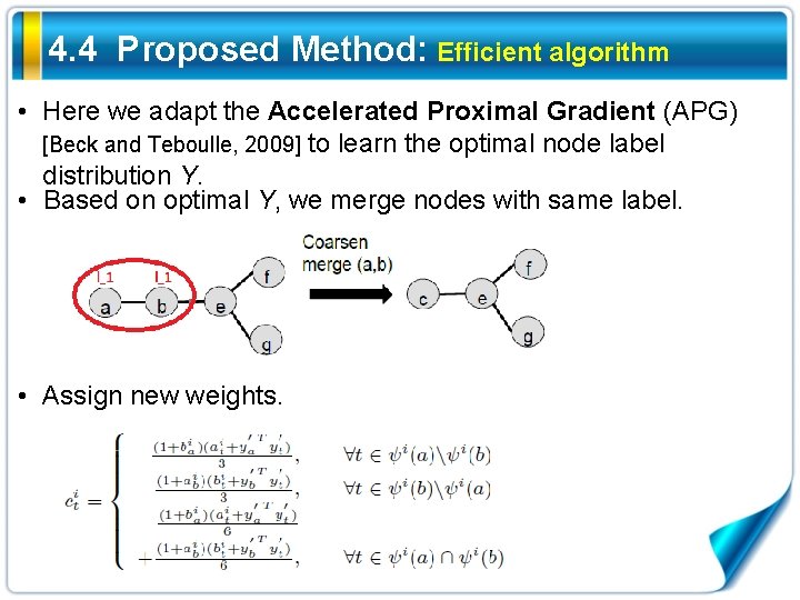
4. 4 Proposed Method: Efficient algorithm • Here we adapt the Accelerated Proximal Gradient (APG) [Beck and Teboulle, 2009] to learn the optimal node label distribution Y. • Based on optimal Y, we merge nodes with same label. • Assign new weights.

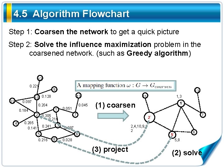
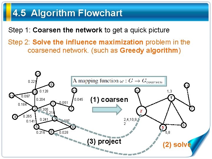
4. 5 Algorithm Flowchart Step 1: Coarsen the network to get a quick picture Step 2: Solve the influence maximization problem in the coarsened network. (such as Greedy algorithm) 12 0. 221 11 0. 097 9 10 0. 128 1 2 3 0. 241 1’ 7 2’ 2, 4, 10, 9, 1 2 0. 097 6 8 1, 3 (1) coarsen 7 5 0. 216 0. 045 0. 051 0. 305 0. 216 0. 265 0. 141 11 13 0. 204 0. 184 4 13 0. 028 6 5’ 5, 8 (3) project (2) solve

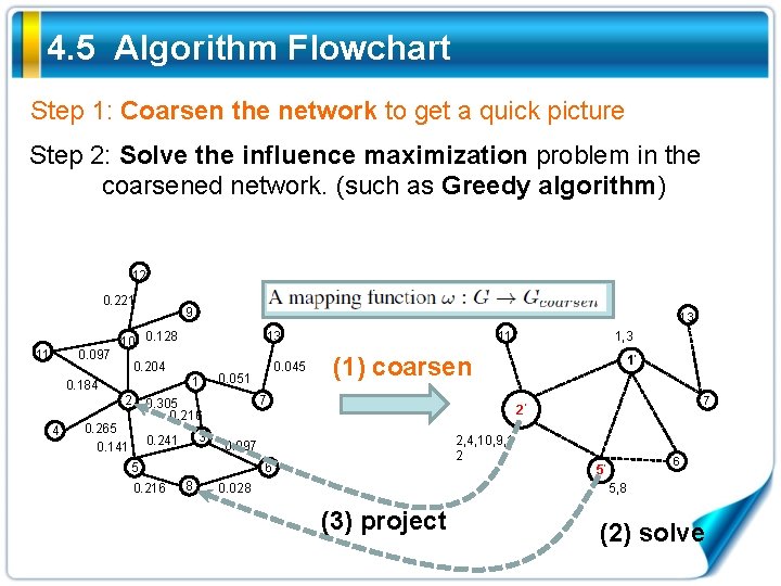
4. 5 Algorithm Flowchart Step 1: Coarsen the network to get a quick picture Step 2: Solve the influence maximization problem in the coarsened network. (such as Greedy algorithm) 12 0. 221 11 0. 097 9 10 0. 128 1 2 3 0. 241 1’ 7 2’ 2, 4, 10, 9, 1 2 0. 097 6 8 1, 3 (1) coarsen 7 5 0. 216 0. 045 0. 051 0. 305 0. 216 0. 265 0. 141 11 13 0. 204 0. 184 4 13 0. 028 6 5’ 5, 8 (3) project (2) solve

4. 5 Algorithm Flowchart Step 1: Coarsen the network to get a quick picture Step 2: Solve the influence maximization problem in the coarsened network. (such as Greedy algorithm) 12 0. 221 11 0. 097 9 10 0. 128 1 2 3 0. 241 1’ 7 2’ 2, 4, 10, 9, 1 2 0. 097 6 8 1, 3 (1) coarsen 7 5 0. 216 0. 045 0. 051 0. 305 0. 216 0. 265 0. 141 11 13 0. 204 0. 184 4 13 0. 028 6 5’ 5, 8 (3) project (2) solve

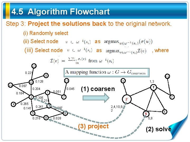
4. 5 Algorithm Flowchart Step 3: Project the solutions back to the original network. (i) Randomly select (ii) Select node as (iii) Select node as , where 12 0. 221 11 0. 097 9 10 0. 128 1 2 3 0. 241 1’ 7 2’ 2, 4, 10, 9, 1 2 0. 097 6 8 1, 3 (1) coarsen 7 5 0. 216 0. 045 0. 051 0. 305 0. 216 0. 265 0. 141 11 13 0. 204 0. 184 4 13 0. 028 6 5’ 5, 8 (3) project (2) solve

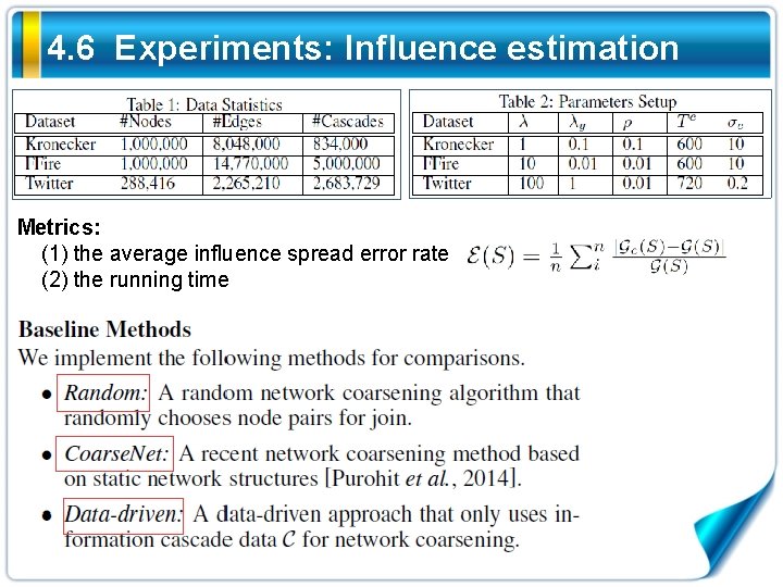
4. 6 Experiments: Influence estimation Metrics: (1) the average influence spread error rate (2) the running time

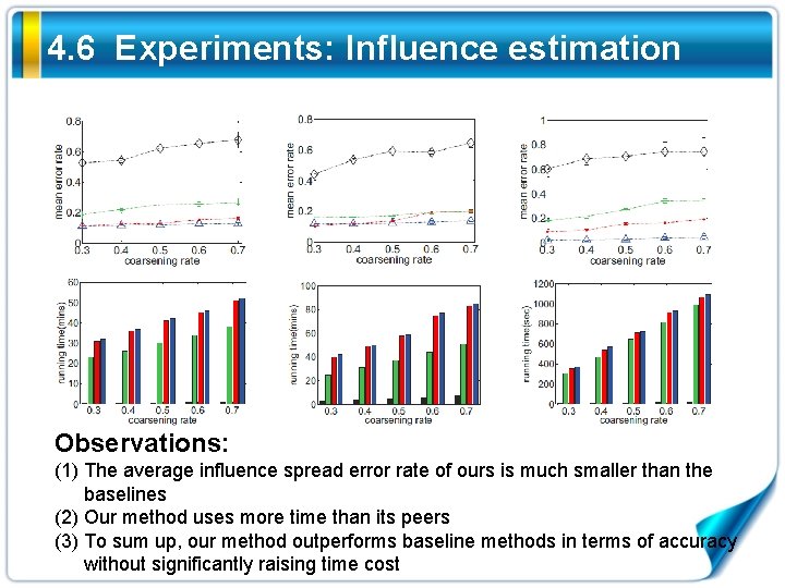
4. 6 Experiments: Influence estimation Observations: (1) The average influence spread error rate of ours is much smaller than the baselines (2) Our method uses more time than its peers (3) To sum up, our method outperforms baseline methods in terms of accuracy without significantly raising time cost

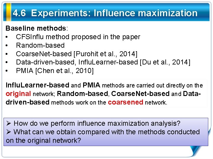
4. 6 Experiments: Influence maximization Baseline methods: • CFSInflu method proposed in the paper • Random-based • Coarse. Net-based [Purohit et al. , 2014] • Data-driven-based, Influ. Learner-based [Du et al. , 2014] • PMIA [Chen et al. , 2010] Influ. Learner-based and PMIA methods are carried out directly on the original network; Random-based, Coarse. Net-based and Datadriven-based methods work on the coarsened network. Ø How do we perform influence maximization analysis? Ø What can we obtain compared with the methods conducted on the original network?

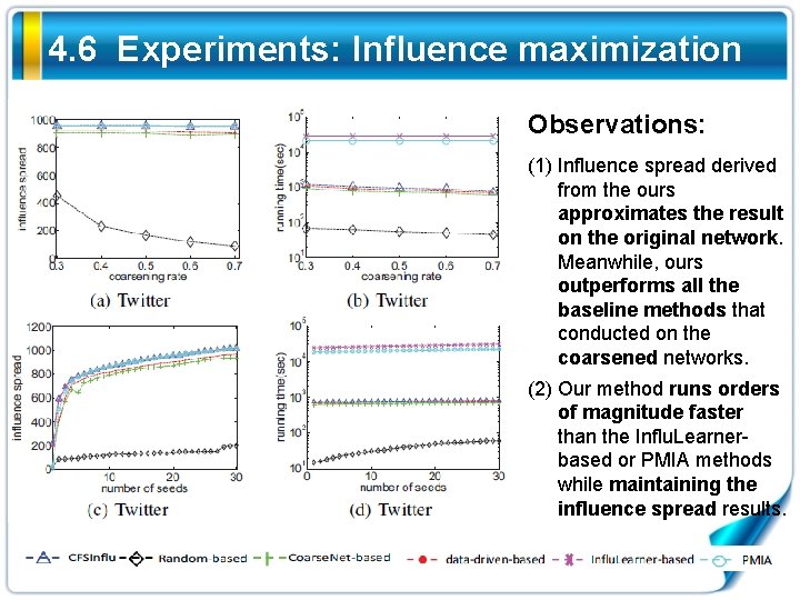
4. 6 Experiments: Influence maximization Observations: (1) Influence spread derived from the ours approximates the result on the original network. Meanwhile, ours outperforms all the baseline methods that conducted on the coarsened networks. (2) Our method runs orders of magnitude faster than the Influ. Learnerbased or PMIA methods while maintaining the influence spread results.

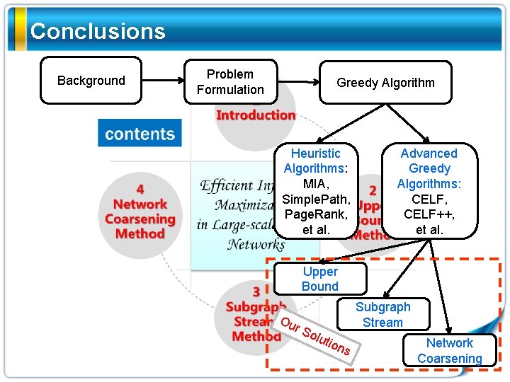
Conclusions Background Problem Formulation Greedy Algorithm Heuristic Algorithms: MIA, Simple. Path, Page. Rank, et al. Advanced Greedy Algorithms: CELF, CELF++, et al. Upper Bound Ou r S olu ti Subgraph Stream ons Network Coarsening

References 1. (TKDE-15) Chuan Zhou, Peng Zhang, Wenyu Zang, and Li Guo. On the Upper Bounds of Spread for Greedy Algorithms in Social Network Influence Maximization. IEEE Transactions on Knowledge and Data Engineering, Vol. 27, No. 10, 2015, 2770 -2783. (CCF-A) 2. (IJCAI-15) Wei-Xue Lu, Peng Zhang, Chuan Zhou, Chunyi Li, and Li Gao. Big Network Influence Maximization: An Incremental Algorithm for Streaming Subgraph Influence Spread Estimation. In Proceedings of the Twenty-Fourth International Joint Conference on Artificial Intelligence, 2076 -2082. (CCF-A) 3. (IJCAI-16) Li Gao, Jia Wu, Hong Yang, Zhi Qiao, Chuan Zhou*, and Yue Hu. Semi-Data-Driven Network Coarsening. In Proceedings of the Twenty-Fifth International Joint Conference on Artificial Intelligence, 1483 -1489. (CCF-A)

Thank You! 周川 Tel: 15101038583 Email: zhouchuan@iie. ac. cn 地址：北京市海淀区闵庄路甲 89号