Efficient Algorithms for Maximum Lifetime Data Gathering and

Efficient Algorithms for Maximum Lifetime Data Gathering and Aggregation in Wireless Sensor Networks Selected from Elsevier: Computer Networks Konstantinos Kalpakis, Koustuv Dasgupta, Parag Namjoshi Presentation by Shu-Ping Lin

Outline n n n n Introduction The Data Gathering Problem Maximum Lifetime Data Gather with Aggregation Greedy CMLDA Incremental CMLDA Experimental Results Conclusions

Outline n n n n Introduction The Data Gathering Problem Maximum Lifetime Data Gather with Aggregation Greedy CMLDA Incremental CMLDA Experimental Results Conclusions

Introduction n Rapid development of sensor results from advances in ¡ ¡ ¡ n Micro-sensor technology Low-power analog/digital electronics Bigger memory size Obstacles arise from ¡ ¡ ¡ Limited energy Computing capabilities Communication resources available

Introduction (cont’d) n n n In this paper authors consider a system of sensors that are homogeneous and highly energy-constrained. Replenishing energy via replacing battery on hundreds of nodes is infeasible. The basic operation is systematic gathering of sensed data to be eventually transmitted to a base station.

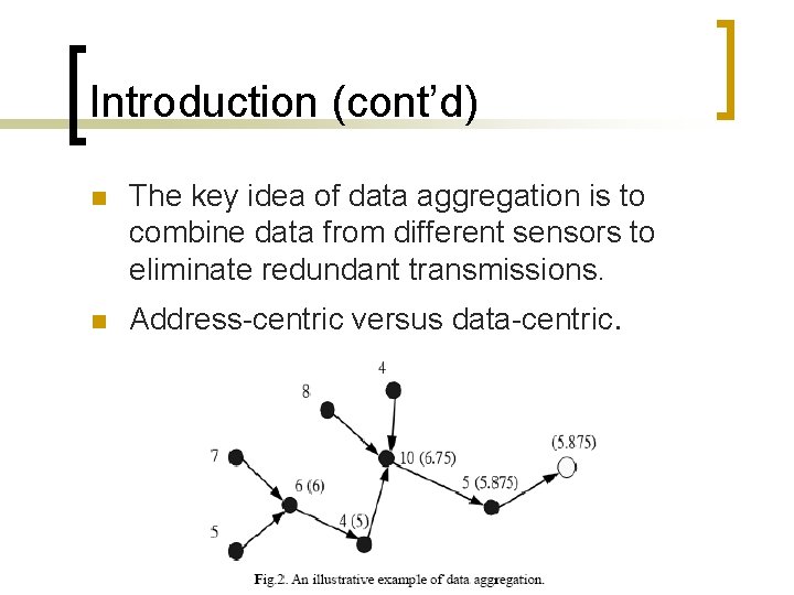
Introduction (cont’d) n n The key idea of data aggregation is to combine data from different sensors to eliminate redundant transmissions. Address-centric versus data-centric.

Introduction (cont’d) n n n This paper derives novel algorithms for data gathering and aggregation in sensor networks. A near-optimal polynomial-time algorithm is proposed, but it is computationally expensive for large sensor networks. Then two heuristics based on GREEDY and INCREASMENTAL concept are derived.

Outline n n n n Introduction The Data Gathering Problem Maximum Lifetime Data Gather with Aggregation Greedy MLDA Incremental MLDA Experimental Results Conclusions

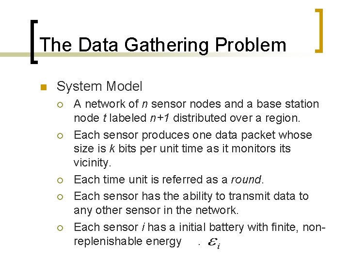
The Data Gathering Problem n System Model ¡ ¡ ¡ A network of n sensor nodes and a base station node t labeled n+1 distributed over a region. Each sensor produces one data packet whose size is k bits per unit time as it monitors its vicinity. Each time unit is referred as a round. Each sensor has the ability to transmit data to any other sensor in the network. Each sensor i has a initial battery with finite, nonreplenishable energy.

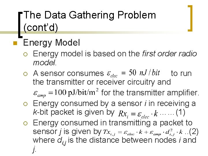
The Data Gathering Problem (cont’d) n Energy Model ¡ ¡ Energy model is based on the first order radio model. A sensor consumes to run the transmitter or receiver circuitry and for the transmitter amplifier. Energy consumed by a sensor i in receiving a k-bit packet is given by ……(1) Energy consumed in transmitting a packet to sensor j is given by. . (2) where di, j is the distance between nodes i and j.

The Data Gathering Problem (cont’d) n Problem Statement ¡ ¡ ¡ Lifetime T of the system to be the number of rounds until the first sensor is drained out. A data gathering schedule specifies how the data packets from all the sensor are collected and transmitted to the base station. The objective of data gathering problem is to find a schedule that maximizes the system lifetime T.

Outline n n n n Introduction The Data Gathering Problem Maximum Lifetime Data Gathering with Aggregation Greedy MLDA Incremental MLDA Experimental Results Conclusions

Maximum Lifetime Data Gathering with Aggregation n Data aggregation performs in-network fusion of data packets in an attempt to minimize the number and size of transmissions and thus save energy. Aggregation can be performed when the data from different sensor are highly correlated. Simplistic assumption ¡ An intermediate sensor can aggregate multiple incoming packets into a single outgoing packet.

Maximum Lifetime Data Gathering with Aggregation (cont’d) n The Maximum Lifetime Data Aggregation (MLDA) problem ¡ Finding a gathering schedule with maximum lifetime, where sensors are permitted to aggregate incoming data packets.

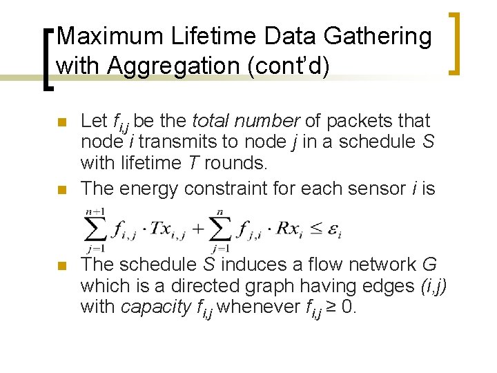
Maximum Lifetime Data Gathering with Aggregation (cont’d) n n n Let fi, j be the total number of packets that node i transmits to node j in a schedule S with lifetime T rounds. The energy constraint for each sensor i is The schedule S induces a flow network G which is a directed graph having edges (i, j) with capacity fi, j whenever fi, j ≥ 0.

Maximum Lifetime Data Gathering with Aggregation (cont’d) n Theorem 1 ¡ n Let S be a schedule with lifetime T, and let G be the flow network induced by S. Then, for each sensor s, the maximum flow from s to the base station t in G is ≥ T. Proof ¡ ¡ Each data packet transmitted from a sensor must reach the base station. In terms of network flows, this implies that sensor s must have a maximum s-t flow of size ≥ T to the base station in the flow network G.

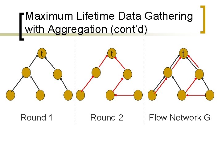
Maximum Lifetime Data Gathering with Aggregation (cont’d) t Round 1 t Round 2 t Flow Network G

Maximum Lifetime Data Gathering with Aggregation (cont’d) n n A necessary condition for a schedule to have lifetime T is that each node in the induced flow network can push flow T to the base station t. Now we must consider the problem of finding a flow network G with maximum T, that allows each sensor to push flow T to the base station, while respecting the energy constraints at all sensor.

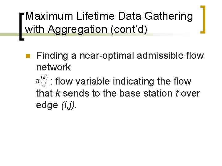
Maximum Lifetime Data Gathering with Aggregation (cont’d) n Finding a near-optimal admissible flow network : flow variable indicating the flow that k sends to the base station t over edge (i, j).

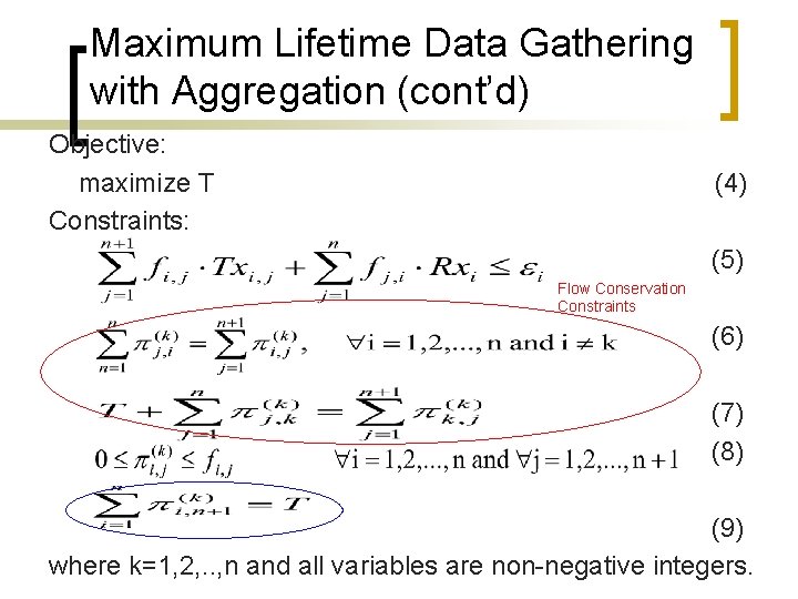
Maximum Lifetime Data Gathering with Aggregation (cont’d) Objective: maximize T Constraints: (4) (5) Flow Conservation Constraints (6) (7) (8) (9) where k=1, 2, . . , n and all variables are non-negative integers.

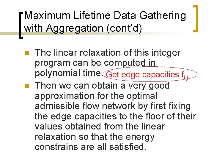
Maximum Lifetime Data Gathering with Aggregation (cont’d) n n The linear relaxation of this integer program can be computed in polynomial time. Get edge capacities fi, j Then we can obtain a very good approximation for the optimal admissible flow network by first fixing the edge capacities to the floor of their values obtained from the linear relaxation so that the energy constrains are all satisfied.

Maximum Lifetime Data Gathering with Aggregation (cont’d) n Finally we solve the linear program (4) subject to constraints (6)-(9) without requiring anymore that the flows are integers.

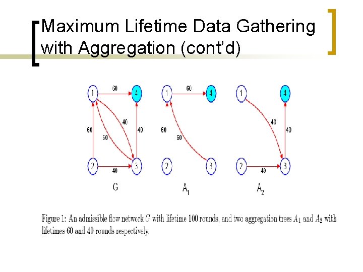
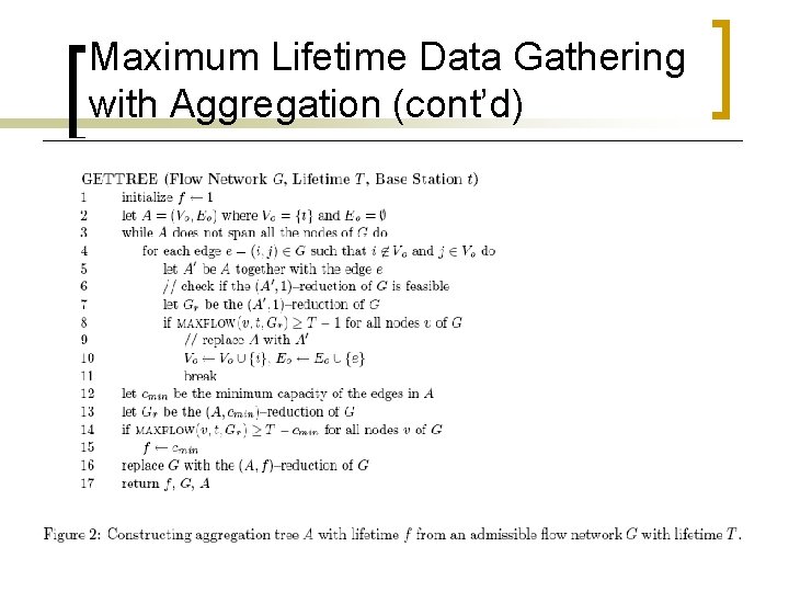
Maximum Lifetime Data Gathering with Aggregation (cont’d) n n n How to get a schedule from an admissible flow network? A schedule is a collection of directed trees that span all the sensors and the base station, with one such tree for each round. These trees are called aggregation trees that may be used for one or more rounds.

Maximum Lifetime Data Gathering with Aggregation (cont’d)

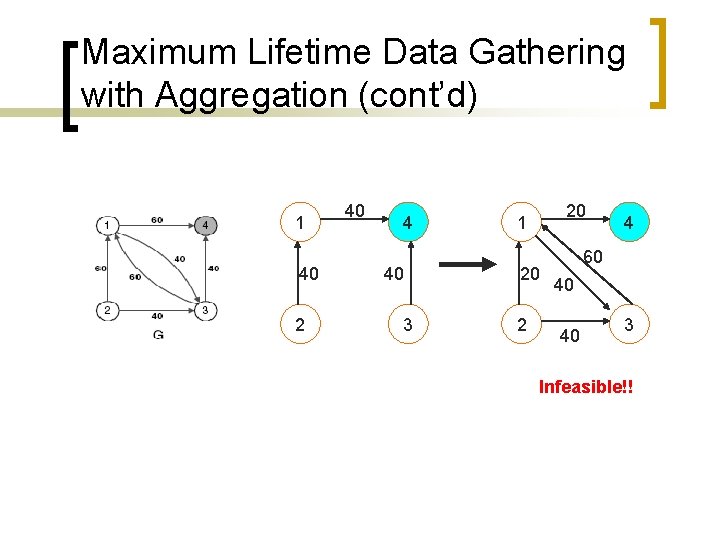
Maximum Lifetime Data Gathering with Aggregation (cont’d) n Definition 1 ¡ ¡ n Given an admissible flow network G with lifetime T and a directed tree A rooted at the base station t with lifetime f. (A, f)-reduction G’ of G is the flow network that results from G after reducing by f, the capacities of all of its edges that are also in A. Definition 2 ¡ An (A, f)-reduction G’ of G is feasible if the maximum flow from node v to the base station t in G’ is ≥ T - f for each node v in G’.

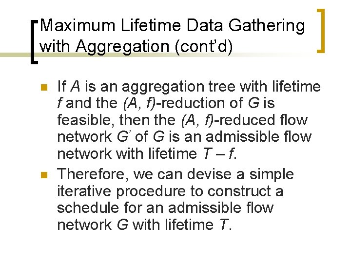
Maximum Lifetime Data Gathering with Aggregation (cont’d) n n If A is an aggregation tree with lifetime f and the (A, f)-reduction of G is feasible, then the (A, f)-reduced flow network G’ of G is an admissible flow network with lifetime T – f. Therefore, we can devise a simple iterative procedure to construct a schedule for an admissible flow network G with lifetime T.

Maximum Lifetime Data Gathering with Aggregation (cont’d) 1 40 2 40 4 40 3 20 1 20 2 4 60 40 40 3 Infeasible!!

Maximum Lifetime Data Gathering with Aggregation (cont’d)

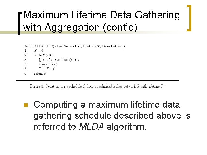
Maximum Lifetime Data Gathering with Aggregation (cont’d) n Computing a maximum lifetime data gathering schedule described above is referred to MLDA algorithm.

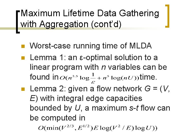
Maximum Lifetime Data Gathering with Aggregation (cont’d) n n n Worst-case running time of MLDA Lemma 1: an ε-optimal solution to a linear program with n variables can be found in time. Lemma 2: given a flow network G = (V, E) with integral edge capacities bounded by U, a maximum s-t flow can be computed in

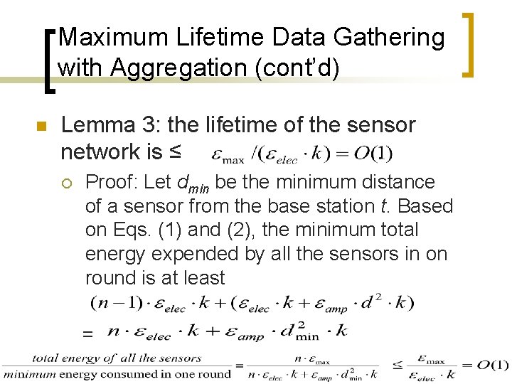
Maximum Lifetime Data Gathering with Aggregation (cont’d) n Lemma 3: the lifetime of the sensor network is ≤. ¡ Proof: Let dmin be the minimum distance of a sensor from the base station t. Based on Eqs. (1) and (2), the minimum total energy expended by all the sensors in on round is at least =

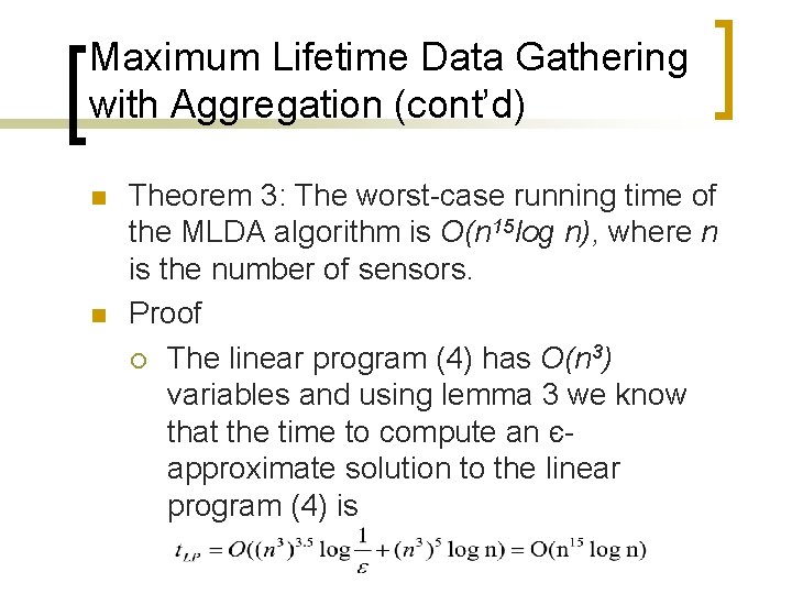
Maximum Lifetime Data Gathering with Aggregation (cont’d) n n Theorem 3: The worst-case running time of the MLDA algorithm is O(n 15 log n), where n is the number of sensors. Proof ¡ The linear program (4) has O(n 3) variables and using lemma 3 we know that the time to compute an єapproximate solution to the linear program (4) is

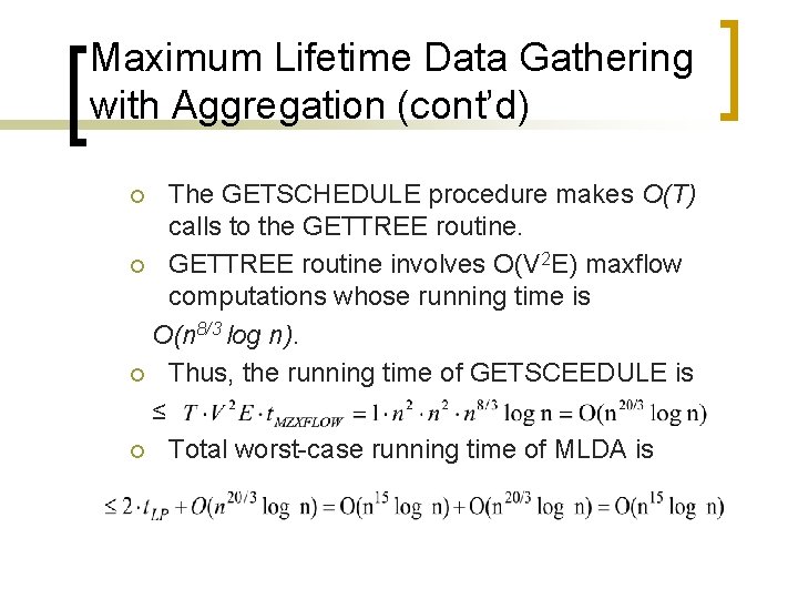
Maximum Lifetime Data Gathering with Aggregation (cont’d) The GETSCHEDULE procedure makes O(T) calls to the GETTREE routine. ¡ GETTREE routine involves O(V 2 E) maxflow computations whose running time is O(n 8/3 log n). ¡ Thus, the running time of GETSCEEDULE is ≤ ¡ Total worst-case running time of MLDA is ¡

Outline n n n n Introduction The Data Gathering Problem Maximum Lifetime Data Gather with Aggregation Greedy CMLDA Incremental CMLDA Experimental Results Conclusions

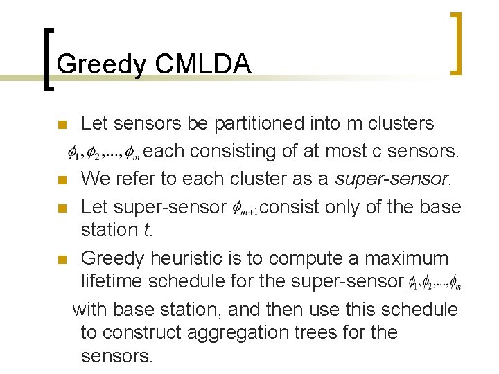
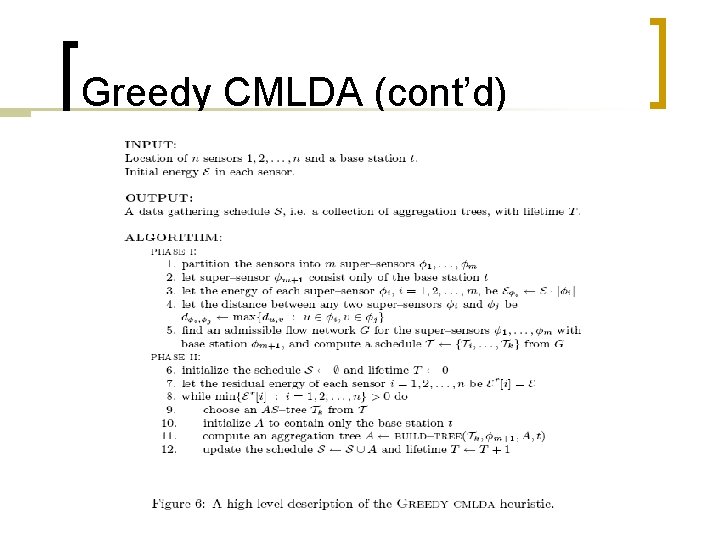
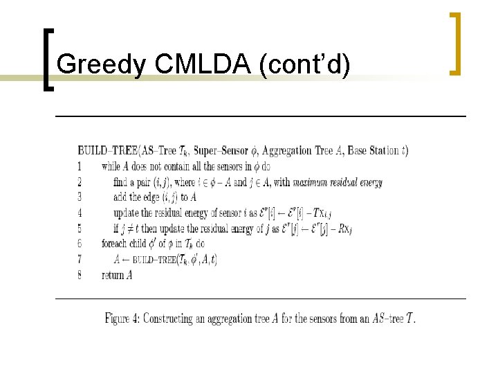
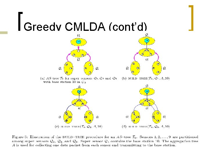
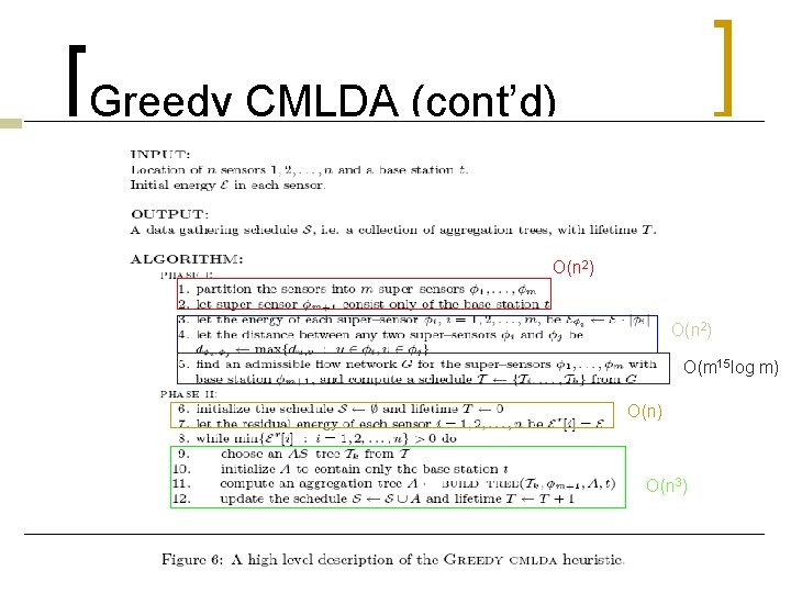
Greedy CMLDA Let sensors be partitioned into m clusters each consisting of at most c sensors. n We refer to each cluster as a super-sensor. n Let super-sensor consist only of the base station t. n Greedy heuristic is to compute a maximum lifetime schedule for the super-sensor with base station, and then use this schedule to construct aggregation trees for the sensors. n

Greedy CMLDA (cont’d)

Greedy CMLDA (cont’d)

Greedy CMLDA (cont’d)

Greedy CMLDA (cont’d) O(n 2) O(m 15 log m) O(n 3)

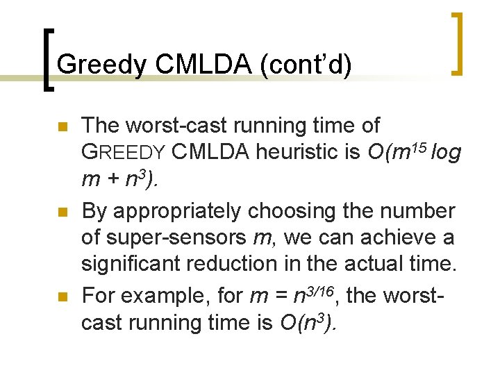
Greedy CMLDA (cont’d) n n n The worst-cast running time of GREEDY CMLDA heuristic is O(m 15 log m + n 3). By appropriately choosing the number of super-sensors m, we can achieve a significant reduction in the actual time. For example, for m = n 3/16, the worstcast running time is O(n 3).

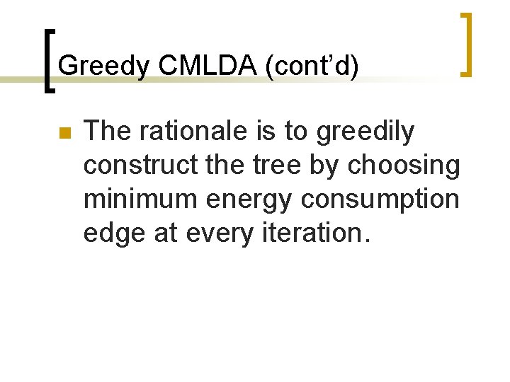
Greedy CMLDA (cont’d) n The rationale is to greedily construct the tree by choosing minimum energy consumption edge at every iteration.

Outline n n n n Introduction The Data Gathering Problem Maximum Lifetime Data Gather with Aggregation Greedy CMLDA Incremental CMLDA Experimental Results Conclusions

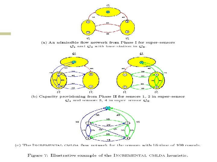
Incremental CMLDA n n n In solving MLDA problem, we are essentially interested in provisioning the (edge) capacities of an admissible flow network G. This proposed heuristic builds such a flow network by incrementally provisioning capacities on its edges. INCREMENTAL MLDA heuristic consists of four phases.

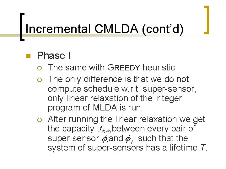
Incremental CMLDA (cont’d) n Phase I ¡ ¡ ¡ The same with GREEDY heuristic The only difference is that we do not compute schedule w. r. t. super-sensor, only linear relaxation of the integer program of MLDA is run. After running the linear relaxation we get the capacity between every pair of super-sensor and , such that the system of super-sensors has a lifetime T.

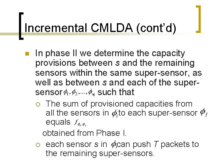
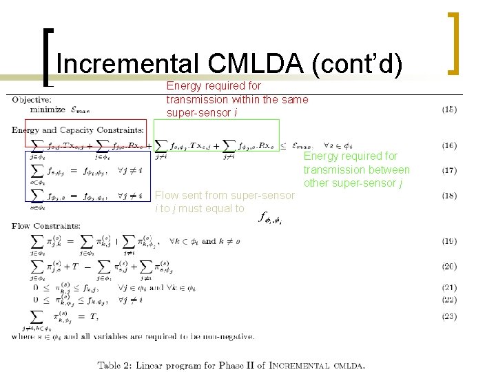
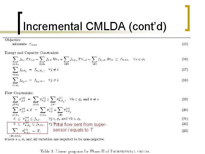
Incremental CMLDA (cont’d) n In phase II we determine the capacity provisions between s and the remaining sensors within the same super-sensor, as well as between s and each of the supersensor , such that The sum of provisioned capacities from all the sensors in to each super-sensor equals obtained from Phase I. ¡ each sensor s in can push T packets to the remaining super-sensors. ¡

Incremental CMLDA (cont’d) n Our objective is to minimize the maximum energy consumed by any sensor within the super-sensor , thereby extending the lifetime of the sensors.

Incremental CMLDA (cont’d) Energy required for transmission within the same super-sensor i Energy required for transmission between other super-sensor j Flow sent from super-sensor i to j must equal to

Incremental CMLDA (cont’d) Total flow sent from supersensor i equals to T

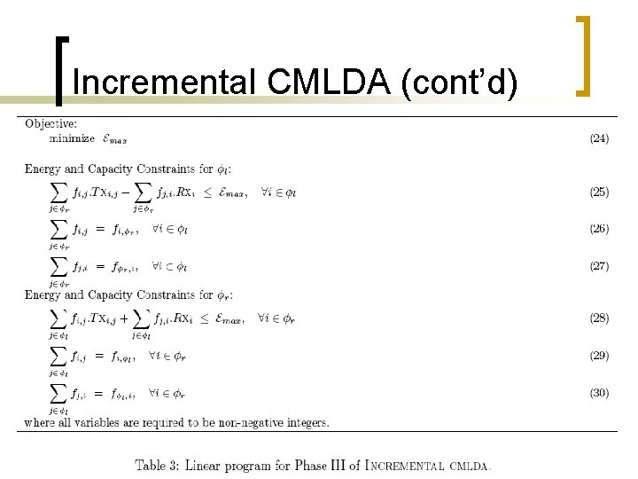
Incremental CMLDA (cont’d) n n From phase II, we obtain the capacity provisions between any sensor s and all other sensors in the same supersensor. In phase III, we need to determine the capacities that need to be provisioned between individual sensors in different super-sensors.

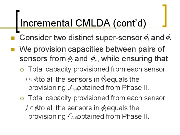
Incremental CMLDA (cont’d) n n Consider two distinct super-sensor and We provision capacities between pairs of sensors from and , while ensuring that ¡ ¡ Total capacity provisioned from each sensor to all the sensors in equals the provisioning obtained from Phase II.

Incremental CMLDA (cont’d)

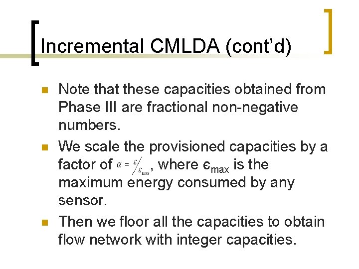
Incremental CMLDA (cont’d) n n n Note that these capacities obtained from Phase III are fractional non-negative numbers. We scale the provisioned capacities by a factor of , where єmax is the maximum energy consumed by any sensor. Then we floor all the capacities to obtain flow network with integer capacities.

Incremental CMLDA (cont’d) n Using this flow network we finally compute the integral system lifetime by MLDA algorithm, and a data gathering schedule S using the GETSCHEDULE algorithm.

Incremental CMLDA (cont’d)

Incremental CMLDA (cont’d) n Worse-case analysis ¡ ¡ ¡ Phase I: O(m 15 log m) Phase II: O(c 5 m 10 log (cm)) Phase III: O(c 10 log c) n Worst-case running time of Incremental CMLDA is n O(m 15 log m) + O(c 5 m 10 log (cm)) + O(c 10 log c)

Outline n n n n Introduction The Data Gathering Problem Maximum Lifetime Data Gather with Aggregation Greedy CMLDA Incremental CMLDA Experimental Results Conclusions

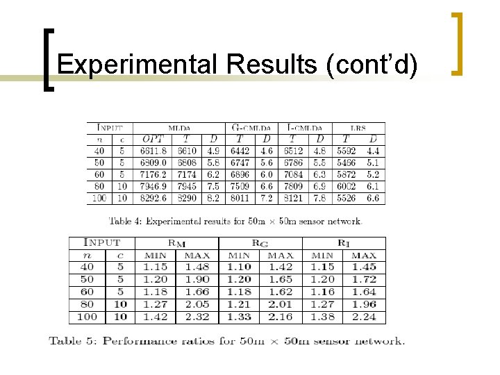
Experimental Results n n n Consider a network of sensors randomly distributed in a 50 m. X 50 m field. The number of sensor in the network is varied to be 40, 50, 60, 80 and 100. Performance ration RM is defined as the ratio of the system lifetime achieved using MLDA to the lifetime given by the LRS protocol.

Experimental Results (cont’d) n n The depth of a sensor v is defined to be its average number of hops from the base station in the schedule. Construct initial cluster ¡ Pick a sensor i farthest from the base station and form a cluster that includes i and its c-1 nearest neighbors.

Experimental Results (cont’d)

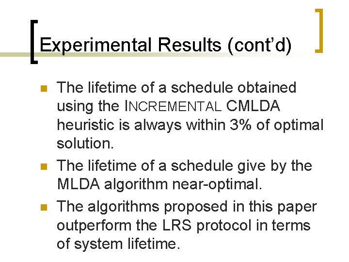
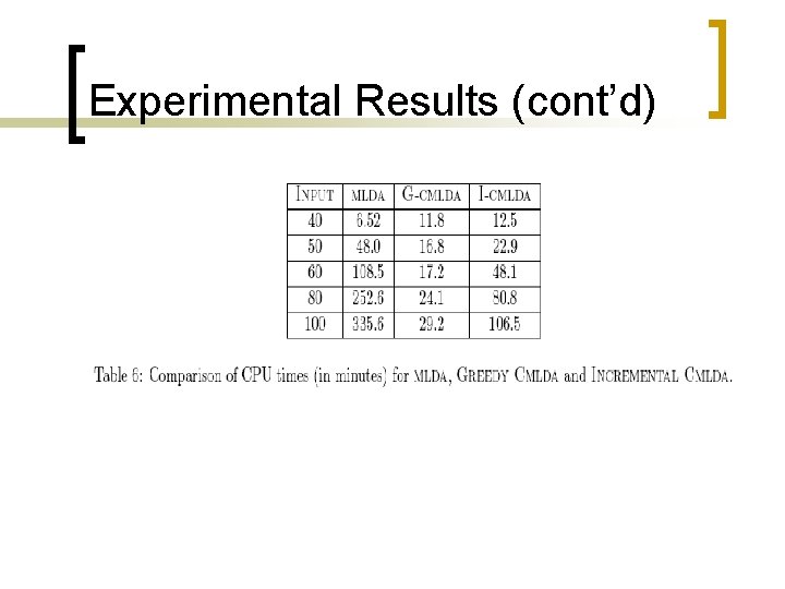
Experimental Results (cont’d) n n n The lifetime of a schedule obtained using the INCREMENTAL CMLDA heuristic is always within 3% of optimal solution. The lifetime of a schedule give by the MLDA algorithm near-optimal. The algorithms proposed in this paper outperform the LRS protocol in terms of system lifetime.

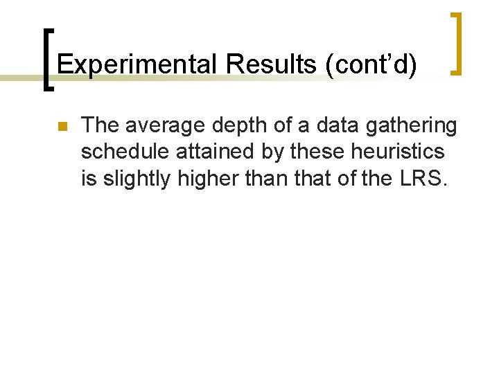
Experimental Results (cont’d) n The average depth of a data gathering schedule attained by these heuristics is slightly higher than that of the LRS.

Experimental Results (cont’d)

Experimental Results (cont’d)

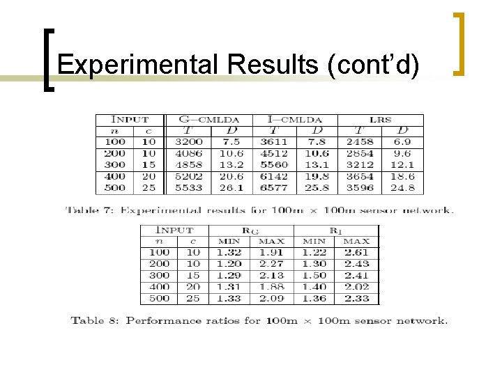
Experimental Results (cont’d) n n The GREEDY and INCREMENTAL CMLDA heuristics significantly outperform the LRS protocol. The average depth of a data gathering schedule attained by these heuristics is only slightly higher than that of the LRS.

Conclusions n n n This paper proposed a polynomial-time near-optimal algorithm (MLDA) for solving the maximum lifetime data gathering problem for sensor networks. Three heuristics are proposed and formulated as linear programming problem. Future research ¡ ¡ Aggregation rate should be included. Depth (delay) constraint is considered.