Effective Reinforcement Learning for Mobile Robots William D

Effective Reinforcement Learning for Mobile Robots William D. Smart & Leslie Pack Kaelbling* Mark J. Buller (mbuller) 14 March 2007 *Proceedings of IEEE International Conference on Robotics and Automation (ICRA 2002), volume 4, pages 3404 -3410, 2002.

Purpose • Programming mobile autonomous robots can be very time consuming – Mapping robot sensor and actuators to programmer understanding can cause misconceptions and control failure • Better: – Define some high level task specification – Let robot learn the implementation • Paper Presents: – “Framework for effectively using reinforcement learning on mobile robots”

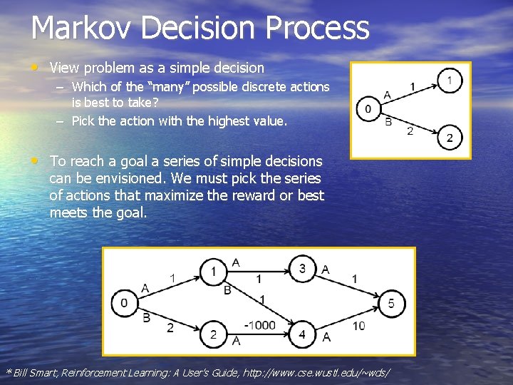
Markov Decision Process • View problem as a simple decision – Which of the “many” possible discrete actions is best to take? – Pick the action with the highest value. • To reach a goal a series of simple decisions can be envisioned. We must pick the series of actions that maximize the reward or best meets the goal. * Bill Smart, Reinforcement Learning: A User’s Guide, http: //www. cse. wustl. edu/~wds/

Markov Decisions Process • A Markov Decision Process (MDP) is represented by • • States S = {s 1, s 2, . . . , sn} Actions A = {a 1, a 2, . . . , am} A reward function R: S×A×S→ℜ A transition function T: S×A→S • An MDP is the structure at the heart of the robot control process. – We often know STATES and ACTIONS – Often need to define TRANSITION function • I. e. Can’t get there from here – Often need to define REWARD function • Optimizes control policy * Bill Smart, Reinforcement Learning: A User’s Guide, http: //www. cse. wustl. edu/~wds/

Reinforcement Learning • An MDP structure can be defined in a number of ways: – Hand coded • Traditional robot control policies – Learned off-line in batch mode • Supervised machine learning – Learned by Reinforcement Learning (RL) • Can observe experiences (s, a, r, s’) • Need to perform actions to generate new experiences • One method is to iteratively learn the “optimal value function” – Q-Learning Algorithm

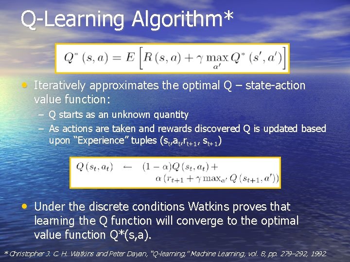
Q-Learning Algorithm* • Iteratively approximates the optimal Q – state-action value function: – Q starts as an unknown quantity – As actions are taken and rewards discovered Q is updated based upon “Experience” tuples (st, at, rt+1, st+1) • Under the discrete conditions Watkins proves that learning the Q function will converge to the optimal value function Q*(s, a). * Christopher J. C. H. Watkins and Peter Dayan, “Q-learning, ” Machine Learning, vol. 8, pp. 279– 292, 1992.

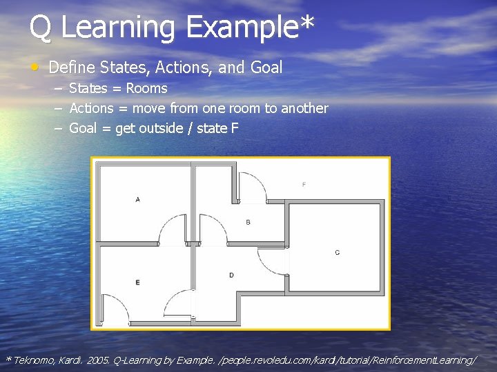
Q Learning Example* • Define States, Actions, and Goal – – – States = Rooms Actions = move from one room to another Goal = get outside / state F * Teknomo, Kardi. 2005. Q-Learning by Example. /people. revoledu. com/kardi/tutorial/Reinforcement. Learning/

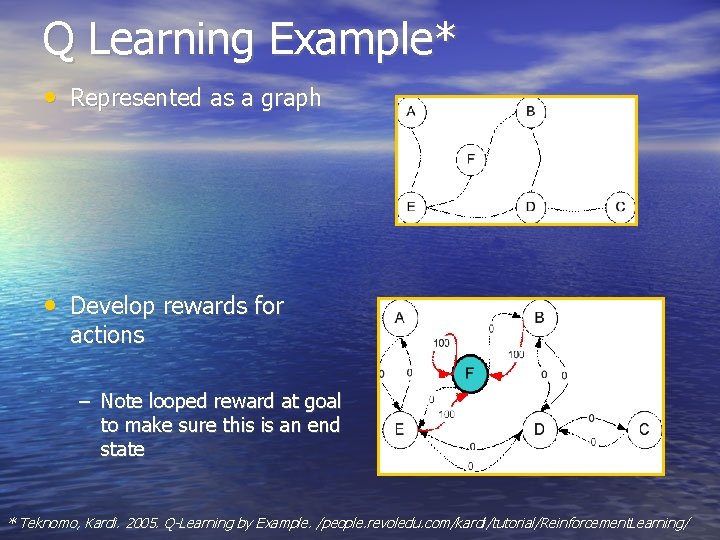
Q Learning Example* • Represented as a graph • Develop rewards for actions – Note looped reward at goal to make sure this is an end state * Teknomo, Kardi. 2005. Q-Learning by Example. /people. revoledu. com/kardi/tutorial/Reinforcement. Learning/

Q Learning Example* • Develop Reward Matrix R R= * Teknomo, Kardi. 2005. Q-Learning by Example. /people. revoledu. com/kardi/tutorial/Reinforcement. Learning/

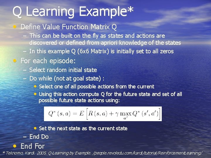
Q Learning Example* • Define Value Function Matrix Q – This can be built on the fly as states and actions are discovered or defined from apriori knowledge of the states – In this example Q (6 x 6 Matrix) is initially set to all zeros • For each episode: – Select random initial state – Do while (not at goal state) : • Select one of all possible actions from the current • Using this action compute Q for the future state and set of all possible future state actions using: • Set the next state as the current state – End Do • End For * Teknomo, Kardi. 2005. Q-Learning by Example. /people. revoledu. com/kardi/tutorial/Reinforcement. Learning/

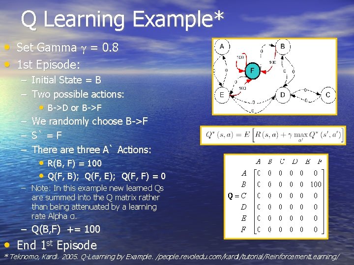
Q Learning Example* • Set Gamma γ = 0. 8 • 1 st Episode: – Initial State = B – Two possible actions: • B->D or B->F – – – We randomly choose B->F S` = F There are three A` Actions: • R(B, F) = 100 • Q(F, B); Q(F, E); Q(F, F) = 0 – Note: In this example new learned Qs are summed into the Q matrix rather than being attenuated by a learning rate Alpha α. – Q(B, F) += 100 • End 1 st Episode * Teknomo, Kardi. 2005. Q-Learning by Example. /people. revoledu. com/kardi/tutorial/Reinforcement. Learning/

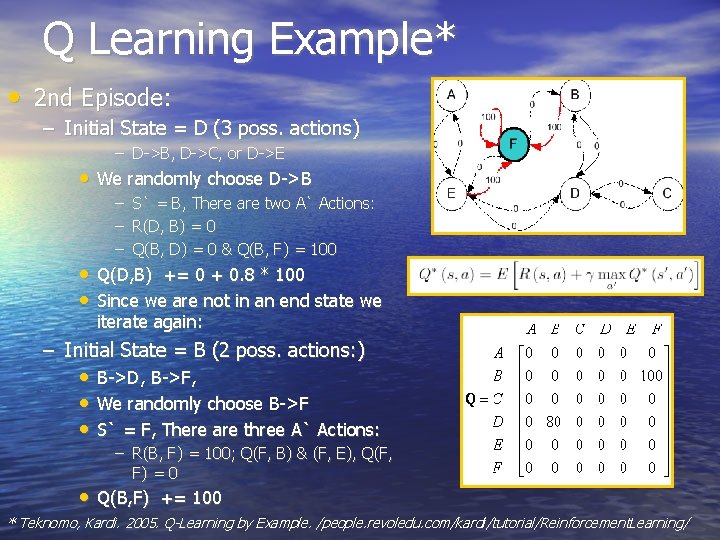
Q Learning Example* • 2 nd Episode: – Initial State = D (3 poss. actions) – D->B, D->C, or D->E • We randomly choose D->B – – – S` = B, There are two A` Actions: R(D, B) = 0 Q(B, D) = 0 & Q(B, F) = 100 • Q(D, B) += 0 + 0. 8 * 100 • Since we are not in an end state we iterate again: – Initial State = B (2 poss. actions: ) • • • B->D, B->F, We randomly choose B->F S` = F, There are three A` Actions: – R(B, F) = 100; Q(F, B) & (F, E), Q(F, F) = 0 • Q(B, F) += 100 * Teknomo, Kardi. 2005. Q-Learning by Example. /people. revoledu. com/kardi/tutorial/Reinforcement. Learning/

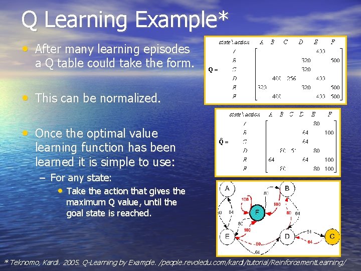
Q Learning Example* • After many learning episodes a Q table could take the form. • This can be normalized. • Once the optimal value learning function has been learned it is simple to use: – For any state: • Take the action that gives the maximum Q value, until the goal state is reached. * Teknomo, Kardi. 2005. Q-Learning by Example. /people. revoledu. com/kardi/tutorial/Reinforcement. Learning/

Reinforcement Learning Applied to Mobile Robots • Reinforcement learning lends itself to mobile robot applications. – Higher-level task description or specification can be thought of in terms of the Reward Function R(s, a) • E. g. Obstacle avoidance problems can be thought of as a reward function that give 1 for reaching the goal -1 for hitting an obstacle and 0 for everything else. – Robot learns the optimal value function through Q learning and applies this function to achieve optimal performance on task

Problems with Straight Application of Q-Learning Algorithm 1) State Space Description of Mobile Robots is best expressed in terms of vectors of real values, not discrete states. • For Q-Learning to converge to the optimal value function discrete states are necessary. 2) Learning is hampered by large state spaces where rewards are sparse • Early stages of learning system choose actions almost arbitrarily • If the system has a very large state space with relatively few rewards the value function approximation will never change until a reward is seen, • This may take some time.

Solutions to Applying Q-Learning to Mobile Robots 1) Limitation of discrete state spaces is overcome by the use of a suitable value-function approximator technique. 1) Early Q-Learning is directed by either an automated or human-in-the-loop control policy.

Value Function Approximator • Value function approximator needs to be chosen with care: – Must never extrapolate but only interpolate. – Extrapolating value function approximators have been shown to fail in even benign situations. • Smart and Kaelbling use the HEDGER algorithm – Checks that the query point is within the training data • Through constructing a “hyper-elliptical hull” around the data and testing for point membership within the hull. (Do we have anyone who can explain this? ) – If query point is within the training data Locally Weighted Regression (LWR) is used to estimate the value function output. – If point is outside of the training data Locally Weighted Averaging (LWA) is used to return a value. • In most cases unless close to the data bounds this would be 0.

Inclusion of Prior Knowledge – The Learning Framework • Learning Occurs in Two Phases – Phase 1: Robot controlled by supplied control policy • Control Code • Human-in-the-loop-control – RL system is NOT in control of the robot • Only observes the states actions and rewards and uses these to update • • the value function approximation Purpose of supplied control policy is to “introduce” the RL system to “interesting” areas of the state space. E. g. where reward is not zero As Q-Learning is “off-policy” it does not learn the control policy but uses experiences to “bootstrap” the value function approximation – Off-policy: “This means that the distribution from which the training samples are drawn has no effect, in the limit, on the policy that is learned. ” – Phase 2: • Once the value function approximation is complete enough: – RL system gains control of the system

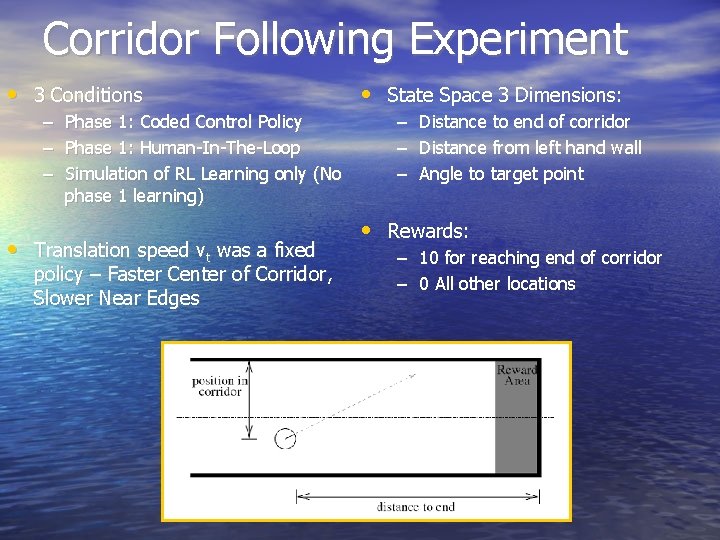
Corridor Following Experiment • 3 Conditions – Phase 1: Coded Control Policy – Phase 1: Human-In-The-Loop – Simulation of RL Learning only (No phase 1 learning) • Translation speed vt was a fixed policy – Faster Center of Corridor, Slower Near Edges • State Space 3 Dimensions: – Distance to end of corridor – Distance from left hand wall – Angle to target point • Rewards: – 10 for reaching end of corridor – 0 All other locations

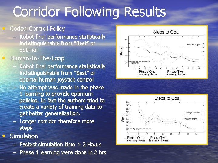
Corridor Following Results • Coded Control Policy – Robot final performance statistically indistinguishable from “Best” or optimal • Human-In-The-Loop – Robot final performance statistically indistinguishable from “Best” or optimal human joystick control – No attempt was made in the phase 1 learning to provide optimum policies. In fact the authors tried to create a variety of training data to get better generalization. – Longer corridor therefore more steps • Simulation – Fastest simulation time > 2 Hours – Phase 1 learning were done in 2 hrs

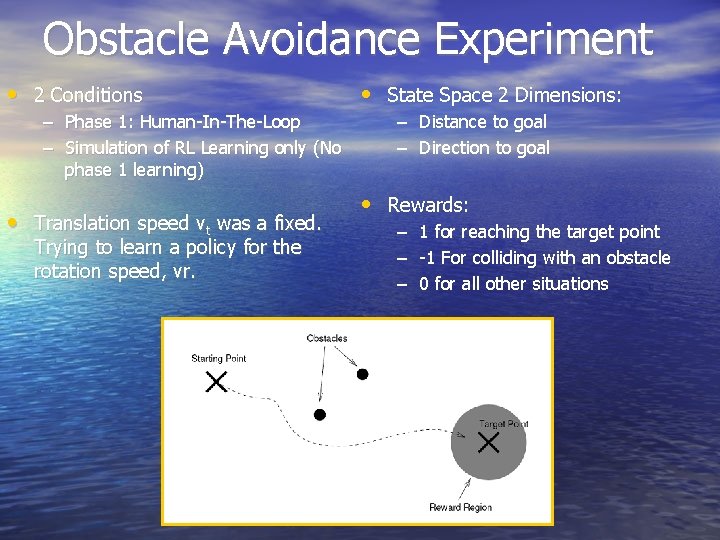
Obstacle Avoidance Experiment • 2 Conditions – Phase 1: Human-In-The-Loop – Simulation of RL Learning only (No phase 1 learning) • Translation speed vt was a fixed. Trying to learn a policy for the rotation speed, vr. • State Space 2 Dimensions: – Distance to goal – Direction to goal • Rewards: – 1 for reaching the target point – -1 For colliding with an obstacle – 0 for all other situations

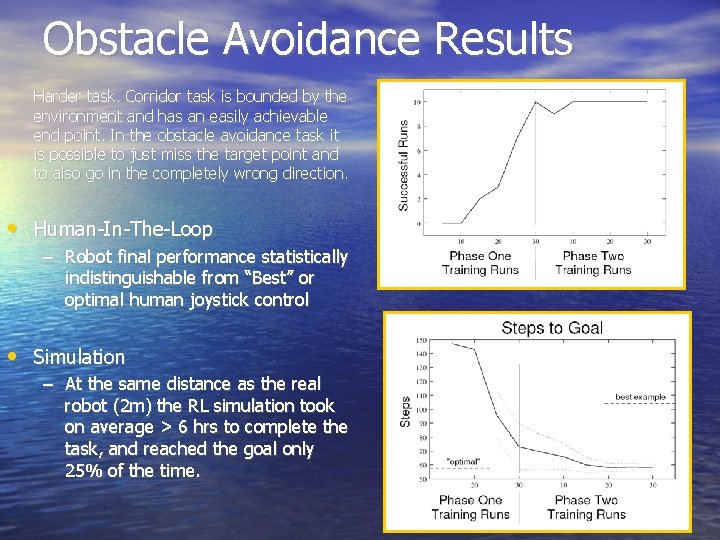
Obstacle Avoidance Results Harder task. Corridor task is bounded by the environment and has an easily achievable end point. In the obstacle avoidance task it is possible to just miss the target point and to also go in the completely wrong direction. • Human-In-The-Loop – Robot final performance statistically indistinguishable from “Best” or optimal human joystick control • Simulation – At the same distance as the real robot (2 m) the RL simulation took on average > 6 hrs to complete the task, and reached the goal only 25% of the time.

Conclusions • Value Function Approximation “Bootstrapping” with example trajectories is much quicker than allowing a RL algorithm struggle to find sparse rewards. • Example trajectories allow the incorporation of human knowledge. • The example trajectories do not need to be the best or near the best. Final performance of the learned system is significantly better than any of the example trajectories. – Generating a breadth of experience for use by the learning system is the important thing. • The framework is capable of learning good control policy more quickly than moderate programmers can hand code control policies

Open Questions • How complex a task can be learned with sparse reward functions? • How does a balance of “good” and “bad” phase one trajectories affect the speed of learning? • Can we automatically determine when to switch to phase 2.

Applications to Roomba Tag • Human in the loop switching to robot control – Isn’t this what we want to do? • Our somewhat generic game definition would provide the basis for: – State dimensions – Reward structure • The learning does not depend upon expert or novice robot controllers. The optimum control policy will be learnt by a broad array of examples from the state dimensions. – Novices may have more negative reward trajectories – Experts may have more positive rewards trajectories – Both sets of trajectories together should make for a better control policy.