Effect Sizes Power Analysis and Statistical Decisions Effect

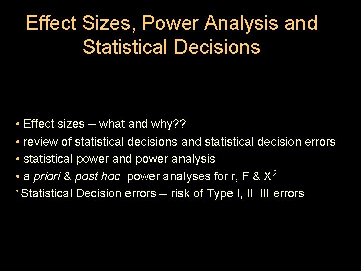
Effect Sizes, Power Analysis and Statistical Decisions • Effect sizes -- what and why? ? • review of statistical decisions and statistical decision errors • statistical power and power analysis • a priori & post hoc power analyses for r, F & X 2 • Statistical Decision errors -- risk of Type I, II III errors

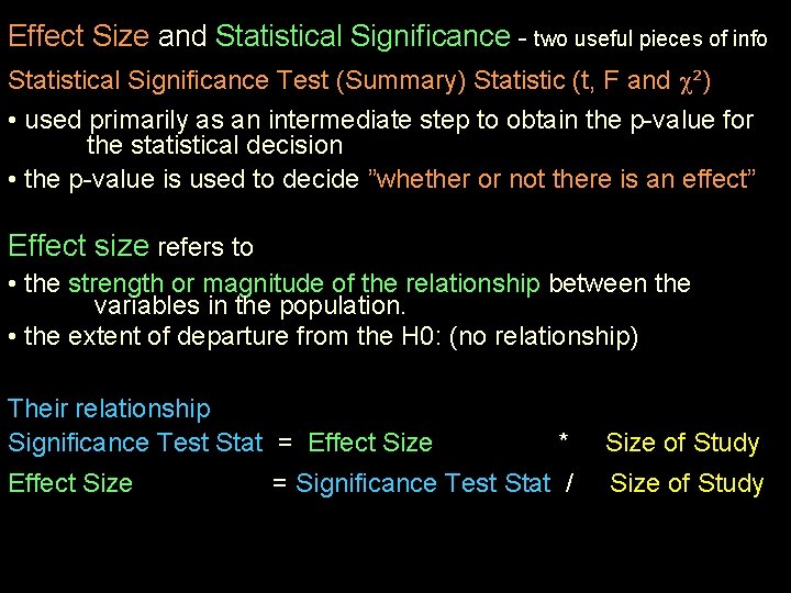
Effect Size and Statistical Significance - two useful pieces of info Statistical Significance Test (Summary) Statistic (t, F and ²) • used primarily as an intermediate step to obtain the p-value for the statistical decision • the p-value is used to decide ”whether or not there is an effect” Effect size refers to • the strength or magnitude of the relationship between the variables in the population. • the extent of departure from the H 0: (no relationship) Their relationship Significance Test Stat = Effect Size * Size of Study = Significance Test Stat / Size of Study

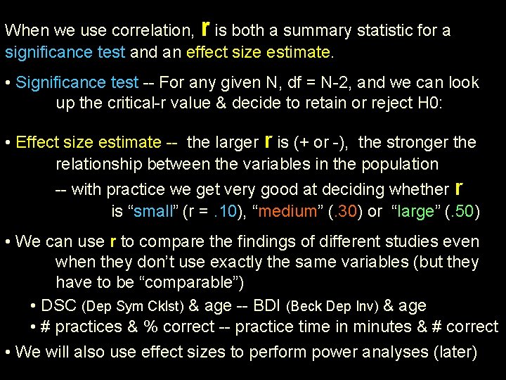
When we use correlation, r is both a summary statistic for a significance test and an effect size estimate. • Significance test -- For any given N, df = N-2, and we can look up the critical-r value & decide to retain or reject H 0: • Effect size estimate -- the larger r is (+ or -), the stronger the relationship between the variables in the population -- with practice we get very good at deciding whether r is “small” (r =. 10), “medium” (. 30) or “large” (. 50) • We can use r to compare the findings of different studies even when they don’t use exactly the same variables (but they have to be “comparable”) • DSC (Dep Sym Cklst) & age -- BDI (Beck Dep Inv) & age • # practices & % correct -- practice time in minutes & # correct • We will also use effect sizes to perform power analyses (later)

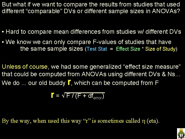
But what if we want to compare the results from studies that used different “comparable” DVs or different sample sizes in ANOVAs? • Hard to compare mean differences from studies w/ different DVs • We know we can only compare F-values of studies that have the sample sizes (Test Stat = Effect Size * Size of Study) Unless of course, we had some generalized “effect size measure” that could be computed from ANOVAs using different DVs & Ns… We do. . . our old buddy r, which can be computed from F r = F / (F + dferror) By the way, when used this way “r” is sometimes called (eta).

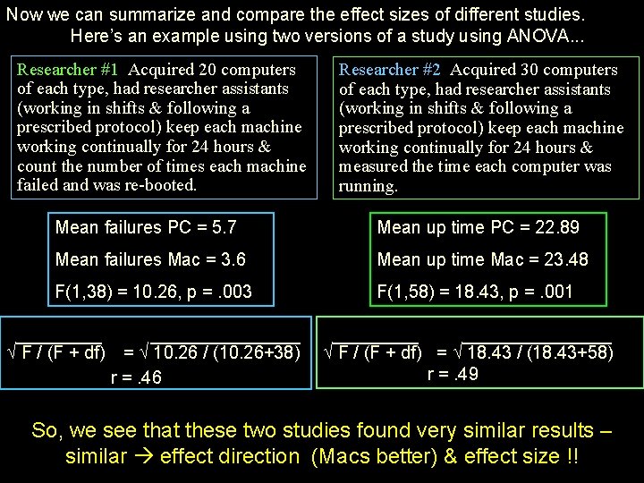
Now we can summarize and compare the effect sizes of different studies. Here’s an example using two versions of a study using ANOVA. . . Researcher #1 Acquired 20 computers of each type, had researcher assistants (working in shifts & following a prescribed protocol) keep each machine working continually for 24 hours & count the number of times each machine failed and was re-booted. Researcher #2 Acquired 30 computers of each type, had researcher assistants (working in shifts & following a prescribed protocol) keep each machine working continually for 24 hours & measured the time each computer was running. Mean failures PC = 5. 7 Mean up time PC = 22. 89 Mean failures Mac = 3. 6 Mean up time Mac = 23. 48 F(1, 38) = 10. 26, p =. 003 F(1, 58) = 18. 43, p =. 001 F / (F + df) = 10. 26 / (10. 26+38) r =. 46 F / (F + df) = 18. 43 / (18. 43+58) r =. 49 So, we see that these two studies found very similar results – similar effect direction (Macs better) & effect size !!

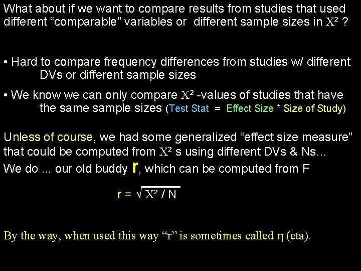
What about if we want to compare results from studies that used different “comparable” variables or different sample sizes in ² ? • Hard to compare frequency differences from studies w/ different DVs or different sample sizes • We know we can only compare ² -values of studies that have the sample sizes (Test Stat = Effect Size * Size of Study) Unless of course, we had some generalized “effect size measure” that could be computed from ² s using different DVs & Ns… We do. . . our old buddy r, which can be computed from F r = ² / N By the way, when used this way “r” is sometimes called (eta).

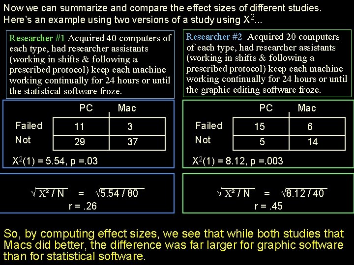
Now we can summarize and compare the effect sizes of different studies. Here’s an example using two versions of a study using X 2. . . Researcher #1 Acquired 40 computers of each type, had researcher assistants (working in shifts & following a prescribed protocol) keep each machine working continually for 24 hours or until the statistical software froze. PC Failed Not Mac 11 3 29 37 X 2(1) = 5. 54, p =. 03 ² / N Researcher #2 Acquired 20 computers of each type, had researcher assistants (working in shifts & following a prescribed protocol) keep each machine working continually for 24 hours or until the graphic editing software froze. = 5. 54 / 80 r =. 26 PC Failed Not Mac 15 6 5 14 X 2(1) = 8. 12, p =. 003 ² / N = 8. 12 / 40 r =. 45 So, by computing effect sizes, we see that while both studies that Macs did better, the difference was far larger for graphic software than for statistical software.

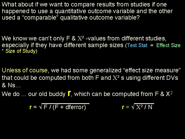
What about if we want to compare results from studies if one happened to use a quantitative outcome variable and the other used a “comparable” qualitative outcome variable? We know we can’t only F & ² -values from different studies, especially if they have different sample sizes (Test Stat = Effect Size * Size of Study) Unless of course, we had some generalized “effect size measure” that could be computed from both F and ² s using different DVs & Ns… We do. . . our old buddy r, which can be computed from F & X 2 r = F / (F + dferror) r = ² / N

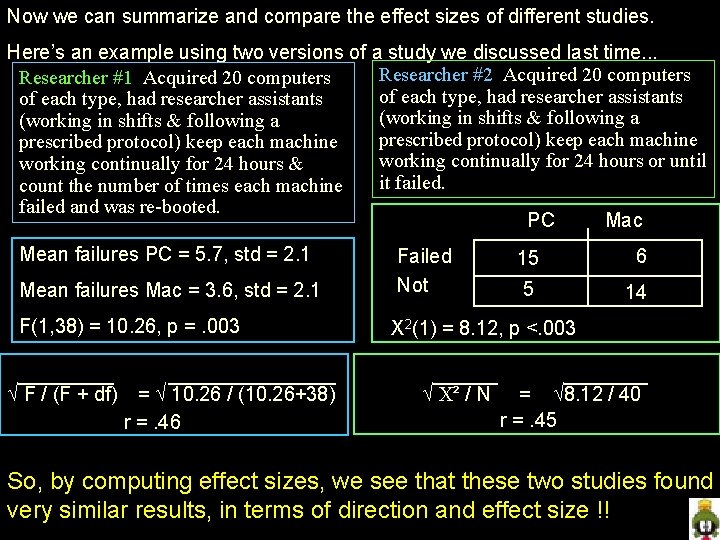
Now we can summarize and compare the effect sizes of different studies. Here’s an example using two versions of a study we discussed last time. . . Researcher #2 Acquired 20 computers Researcher #1 Acquired 20 computers of each type, had researcher assistants (working in shifts & following a prescribed protocol) keep each machine working continually for 24 hours or until working continually for 24 hours & it failed. count the number of times each machine failed and was re-booted. PC Mac Mean failures PC = 5. 7, std = 2. 1 15 6 5 14 Mean failures Mac = 3. 6, std = 2. 1 Failed Not F(1, 38) = 10. 26, p =. 003 X 2(1) = 8. 12, p <. 003 F / (F + df) = 10. 26 / (10. 26+38) r =. 46 ² / N = 8. 12 / 40 r =. 45 So, by computing effect sizes, we see that these two studies found very similar results, in terms of direction and effect size !!

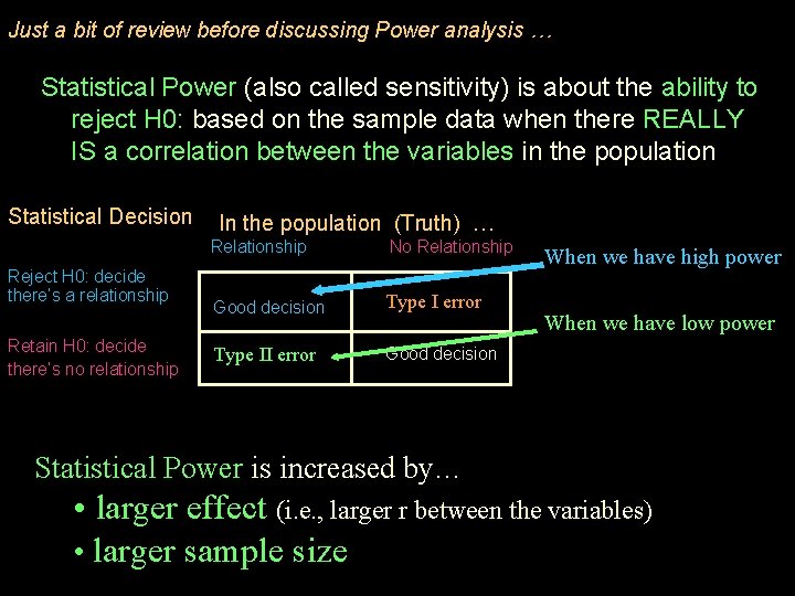
Just a bit of review before discussing Power analysis … Statistical Power (also called sensitivity) is about the ability to reject H 0: based on the sample data when there REALLY IS a correlation between the variables in the population Statistical Decision Reject H 0: decide there’s a relationship Retain H 0: decide there’s no relationship In the population (Truth) … Relationship No Relationship Good decision Type I error Type II error Good decision When we have high power When we have low power Statistical Power is increased by… • larger effect (i. e. , larger r between the variables) • larger sample size

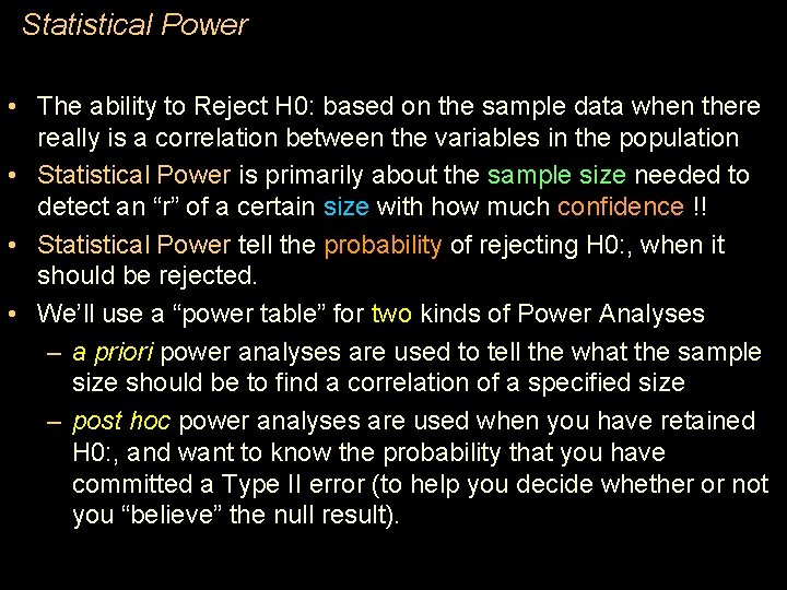
Statistical Power • The ability to Reject H 0: based on the sample data when there really is a correlation between the variables in the population • Statistical Power is primarily about the sample size needed to detect an “r” of a certain size with how much confidence !! • Statistical Power tell the probability of rejecting H 0: , when it should be rejected. • We’ll use a “power table” for two kinds of Power Analyses – a priori power analyses are used to tell the what the sample size should be to find a correlation of a specified size – post hoc power analyses are used when you have retained H 0: , and want to know the probability that you have committed a Type II error (to help you decide whether or not you “believe” the null result).

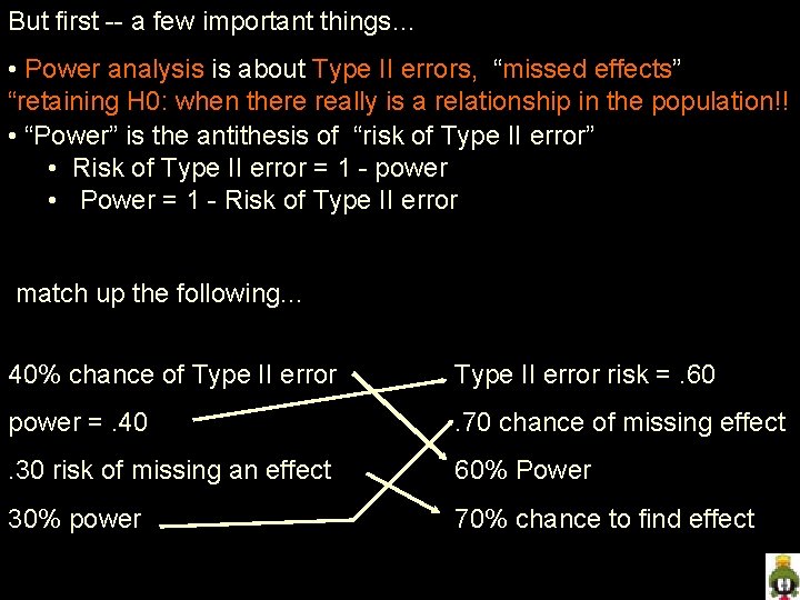
But first -- a few important things… • Power analysis is about Type II errors, “missed effects” “retaining H 0: when there really is a relationship in the population!! • “Power” is the antithesis of “risk of Type II error” • Risk of Type II error = 1 - power • Power = 1 - Risk of Type II error match up the following. . . 40% chance of Type II error risk =. 60 power =. 40 . 70 chance of missing effect . 30 risk of missing an effect 60% Power 30% power 70% chance to find effect

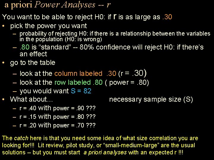
a priori Power Analyses -- r You want to be able to reject H 0: if r is as large as. 30 • pick the power you want – probability of rejecting H 0: if there is a relationship between the variables in the population (H 0: is wrong) –. 80 is “standard” -- 80% confidence will reject H 0: if there’s an effect • go to the table – look at the column labeled. 30 (r =. 30) – look at the row labeled. 80 ( power =. 80) – you would want S = 82 • What about… necessary sample size (S) – r =. 40 with power =. 90 ? ? ? – r =. 15 with power =. 80 ? ? ? – r =. 20 with power =. 70 ? ? ? The catch here is that you need some idea of what size correlation you are looking for!!! Lit review, pilot study, or “small-medium-large” are the usual solutions -- but you must start a priori analyses with an expected r !!!

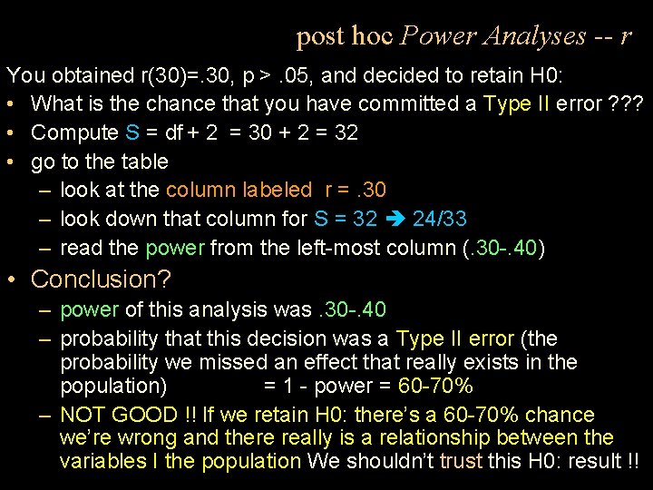
post hoc Power Analyses -- r You obtained r(30)=. 30, p >. 05, and decided to retain H 0: • What is the chance that you have committed a Type II error ? ? ? • Compute S = df + 2 = 30 + 2 = 32 • go to the table – look at the column labeled r =. 30 – look down that column for S = 32 24/33 – read the power from the left-most column (. 30 -. 40) • Conclusion? – power of this analysis was. 30 -. 40 – probability that this decision was a Type II error (the probability we missed an effect that really exists in the population) = 1 - power = 60 -70% – NOT GOOD !! If we retain H 0: there’s a 60 -70% chance we’re wrong and there really is a relationship between the variables I the population We shouldn’t trust this H 0: result !!

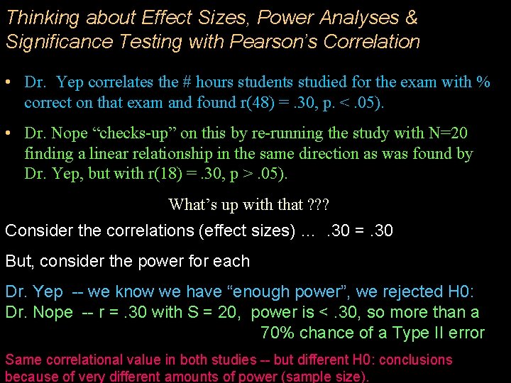
Thinking about Effect Sizes, Power Analyses & Significance Testing with Pearson’s Correlation • Dr. Yep correlates the # hours students studied for the exam with % correct on that exam and found r(48) =. 30, p. <. 05). • Dr. Nope “checks-up” on this by re-running the study with N=20 finding a linear relationship in the same direction as was found by Dr. Yep, but with r(18) =. 30, p >. 05). What’s up with that ? ? ? Consider the correlations (effect sizes) …. 30 =. 30 But, consider the power for each Dr. Yep -- we know we have “enough power”, we rejected H 0: Dr. Nope -- r =. 30 with S = 20, power is <. 30, so more than a 70% chance of a Type II error Same correlational value in both studies -- but different H 0: conclusions because of very different amounts of power (sample size).

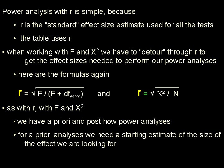
Power analysis with r is simple, because • r is the “standard” effect size estimate used for all the tests • the table uses r • when working with F and X 2 we have to “detour” through r to get the effect sizes needed to perform our power analyses • here are the formulas again r = F / (F + dferror) and r = ² / N • as with r, with F and X 2 • we have a priori and post how power analyses • for a priori analyses we need a starting estimate of the size of the effect we are looking for

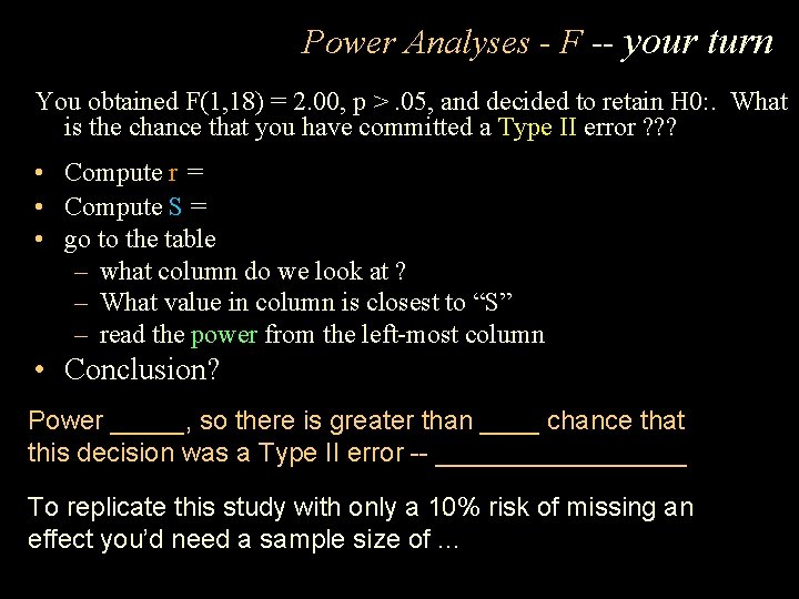
Power Analyses - F -- your turn You obtained F(1, 18) = 2. 00, p >. 05, and decided to retain H 0: . What is the chance that you have committed a Type II error ? ? ? • Compute r = • Compute S = • go to the table – what column do we look at ? – What value in column is closest to “S” – read the power from the left-most column • Conclusion? Power _____, so there is greater than ____ chance that this decision was a Type II error -- _________ To replicate this study with only a 10% risk of missing an effect you’d need a sample size of. . .

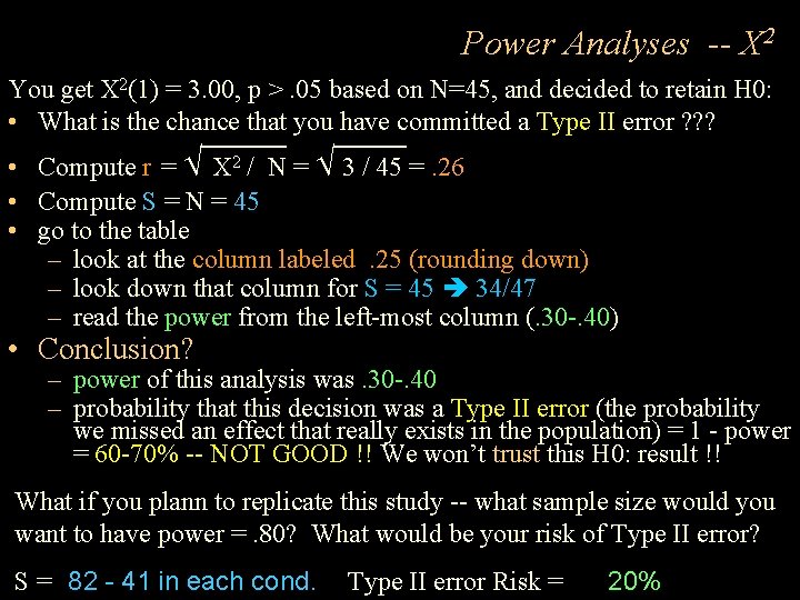
Power Analyses -- X 2 You get X 2(1) = 3. 00, p >. 05 based on N=45, and decided to retain H 0: • What is the chance that you have committed a Type II error ? ? ? • Compute r = X 2 / N = 3 / 45 =. 26 • Compute S = N = 45 • go to the table – look at the column labeled. 25 (rounding down) – look down that column for S = 45 34/47 – read the power from the left-most column (. 30 -. 40) • Conclusion? – power of this analysis was. 30 -. 40 – probability that this decision was a Type II error (the probability we missed an effect that really exists in the population) = 1 - power = 60 -70% -- NOT GOOD !! We won’t trust this H 0: result !! What if you plann to replicate this study -- what sample size would you want to have power =. 80? What would be your risk of Type II error? S = 82 - 41 in each cond. Type II error Risk = 20%

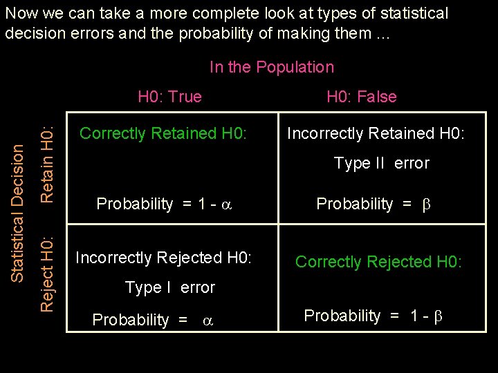
Now we can take a more complete look at types of statistical decision errors and the probability of making them. . . In the Population Retain H 0: Reject H 0: Statistical Decision H 0: True Correctly Retained H 0: False Incorrectly Retained H 0: Type II error Probability = 1 - Incorrectly Rejected H 0: Probability = Correctly Rejected H 0: Type I error Probability = 1 -

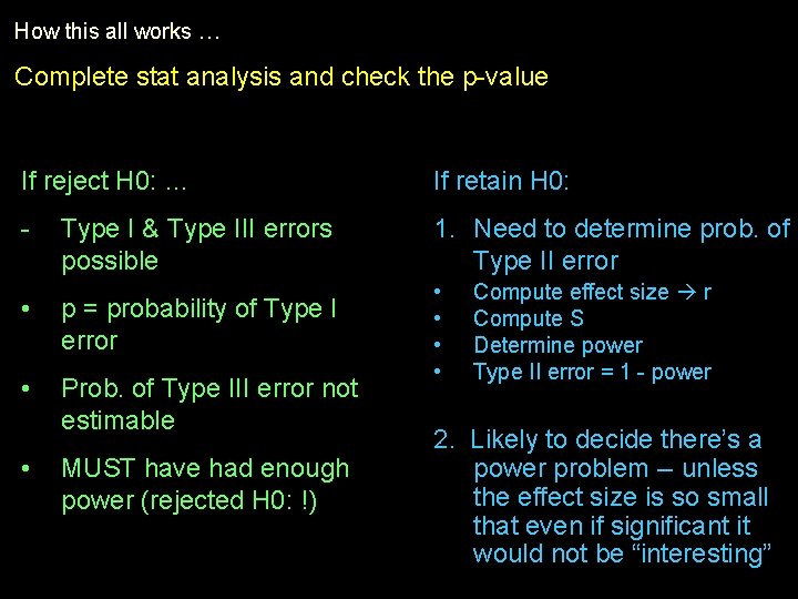
How this all works … Complete stat analysis and check the p-value If reject H 0: … If retain H 0: - Type I & Type III errors possible 1. Need to determine prob. of Type II error • p = probability of Type I error • Prob. of Type III error not estimable • • • MUST have had enough power (rejected H 0: !) Compute effect size r Compute S Determine power Type II error = 1 - power 2. Likely to decide there’s a power problem -- unless the effect size is so small that even if significant it would not be “interesting”

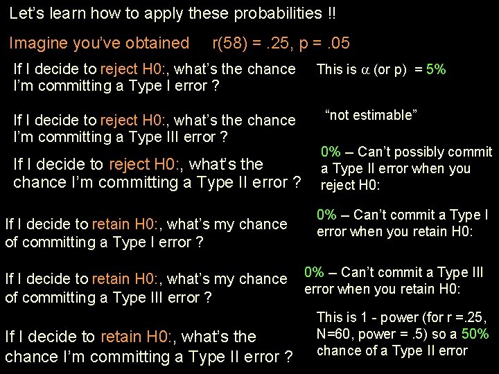
Let’s learn how to apply these probabilities !! Imagine you’ve obtained r(58) =. 25, p =. 05 If I decide to reject H 0: , what’s the chance I’m committing a Type I error ? If I decide to reject H 0: , what’s the chance I’m committing a Type III error ? If I decide to reject H 0: , what’s the chance I’m committing a Type II error ? If I decide to retain H 0: , what’s my chance of committing a Type III error ? If I decide to retain H 0: , what’s the chance I’m committing a Type II error ? This is (or p) = 5% “not estimable” 0% -- Can’t possibly commit a Type II error when you reject H 0: 0% -- Can’t commit a Type I error when you retain H 0: 0% -- Can’t commit a Type III error when you retain H 0: This is 1 - power (for r =. 25, N=60, power =. 5) so a 50% chance of a Type II error