EFFECT SIZES POWER ANALYSIS 8 CONTENTS Different forms

EFFECT SIZES & POWER ANALYSIS 8

CONTENTS Different forms of effect sizes Power Analysis

What is an effect size? Natural effect size Standardized effect size DIFFERENT FORMS OF EFFECT SIZE Normalized effect size Variance explained

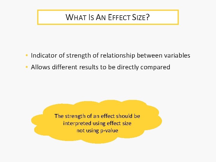
WHAT IS AN EFFECT SIZE? • Indicator of strength of relationship between variables • Allows different results to be directly compared The strength of an effect should be interpreted using effect size not using p-value

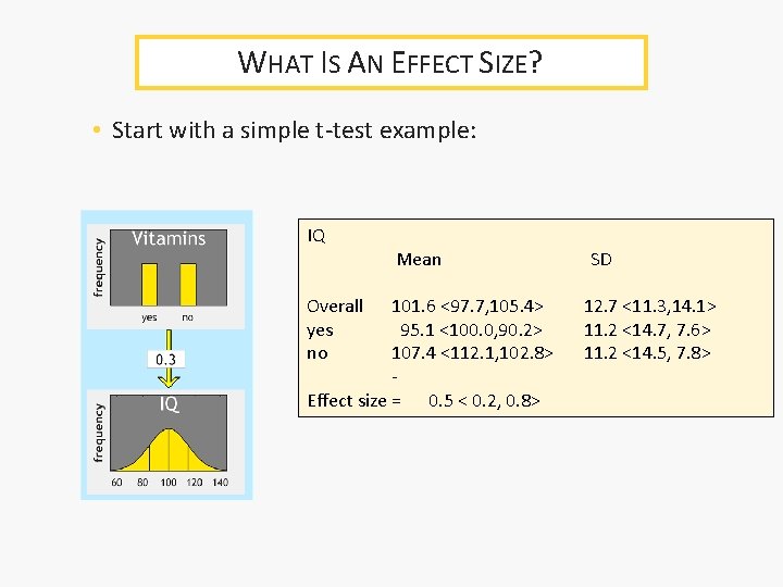
WHAT IS AN EFFECT SIZE? • Start with a simple t-test example: IQ Overall yes no Mean 101. 6 <97. 7, 105. 4> 95. 1 <100. 0, 90. 2> 107. 4 <112. 1, 102. 8> Effect size = 0. 5 < 0. 2, 0. 8> SD 12. 7 <11. 3, 14. 1> 11. 2 <14. 7, 7. 6> 11. 2 <14. 5, 7. 8>

WHAT IS AN EFFECT SIZE? • Effect size = how strong the relationship is • 4 ways ‣ Natural ‣ Standardized ‣ Normalized ‣ Variance explained

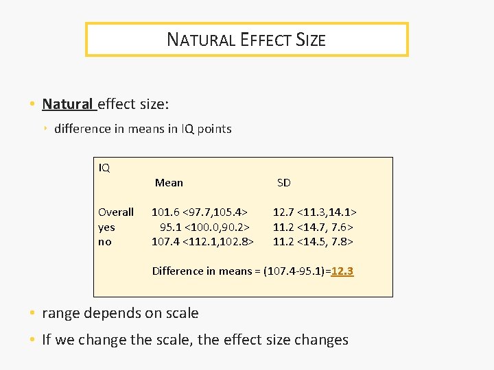
NATURAL EFFECT SIZE • Natural effect size: ‣ difference in means in IQ points IQ Overall yes no Mean 101. 6 <97. 7, 105. 4> 95. 1 <100. 0, 90. 2> 107. 4 <112. 1, 102. 8> SD 12. 7 <11. 3, 14. 1> 11. 2 <14. 7, 7. 6> 11. 2 <14. 5, 7. 8> Difference in means = (107. 4 -95. 1)=12. 3 • range depends on scale • If we change the scale, the effect size changes

NATURAL EFFECT SIZE • Good for cases where there is a real-world scale already in use and widely recognized ‣ “Taking vitamins increases IQ by 12 points” ‣ IQ scale is known • Otherwise it is not easy to make any sense of the number ‣ “Taking vitamins decreases perfectionism by 4 points” ‣ perfectionism scale is not known

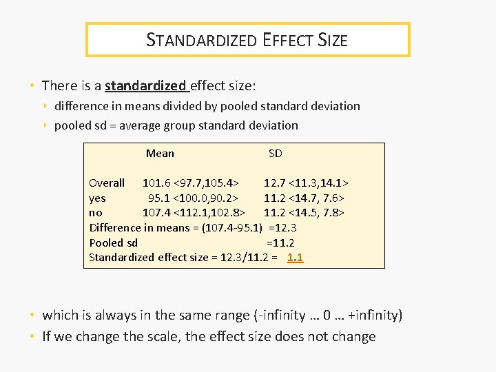
STANDARDIZED EFFECT SIZE • There is a standardized effect size: ‣ difference in means divided by pooled standard deviation ‣ pooled sd = average group standard deviation Mean SD Overall 101. 6 <97. 7, 105. 4> 12. 7 <11. 3, 14. 1> yes 95. 1 <100. 0, 90. 2> 11. 2 <14. 7, 7. 6> no 107. 4 <112. 1, 102. 8> 11. 2 <14. 5, 7. 8> Difference in means = (107. 4 -95. 1) =12. 3 Pooled sd =11. 2 Standardized effect size = 12. 3/11. 2 = 1. 1 • which is always in the same range (-infinity … 0 … +infinity) • If we change the scale, the effect size does not change

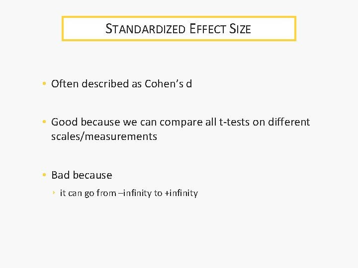
STANDARDIZED EFFECT SIZE • Often described as Cohen’s d • Good because we can compare all t-tests on different scales/measurements • Bad because ‣ it can go from –infinity to +infinity

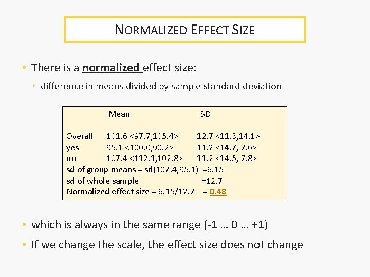
NORMALIZED EFFECT SIZE • There is a normalized effect size: ‣ difference in means divided by sample standard deviation Mean SD Overall 101. 6 <97. 7, 105. 4> 12. 7 <11. 3, 14. 1> yes 95. 1 <100. 0, 90. 2> 11. 2 <14. 7, 7. 6> no 107. 4 <112. 1, 102. 8> 11. 2 <14. 5, 7. 8> sd of group means = sd(107. 4, 95. 1) =6. 15 sd of whole sample =12. 7 Normalized effect size = 6. 15/12. 7 = 0. 48 • which is always in the same range (-1 … 0 … +1) • If we change the scale, the effect size does not change

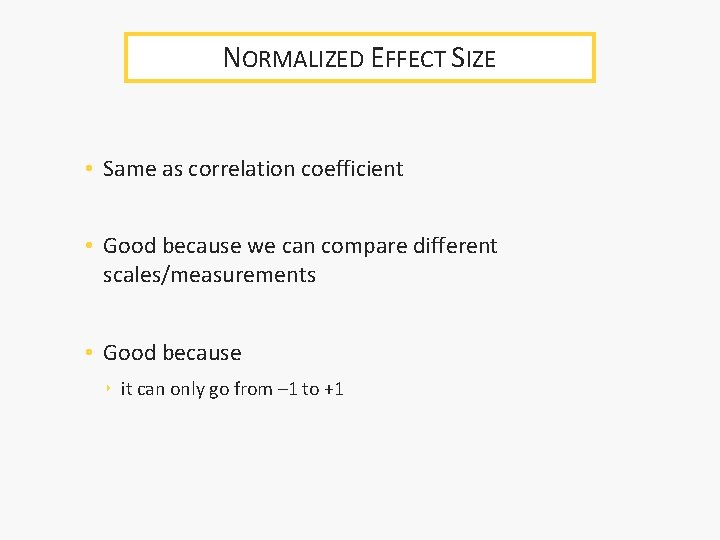
NORMALIZED EFFECT SIZE • Same as correlation coefficient • Good because we can compare different scales/measurements • Good because ‣ it can only go from – 1 to +1

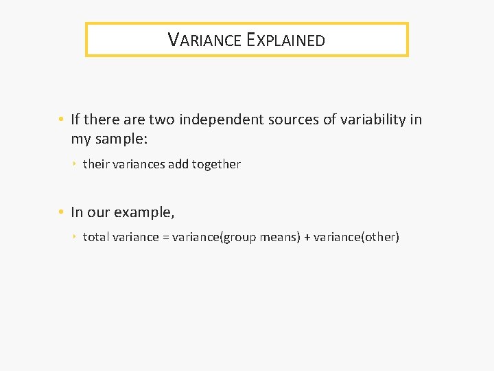
VARIANCE EXPLAINED • If there are two independent sources of variability in my sample: ‣ their variances add together • In our example, ‣ total variance = variance(group means) + variance(other)

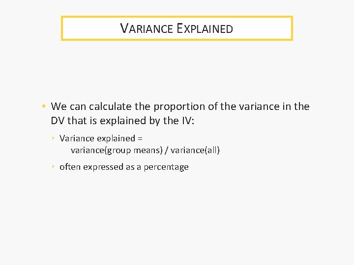
VARIANCE EXPLAINED • We can calculate the proportion of the variance in the DV that is explained by the IV: ‣ Variance explained = variance(group means) / variance(all) ‣ often expressed as a percentage

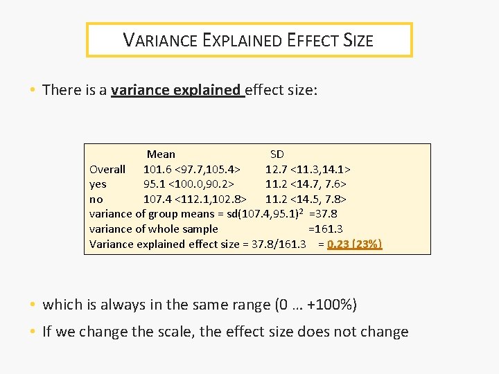
VARIANCE EXPLAINED EFFECT SIZE • There is a variance explained effect size: Mean SD Overall 101. 6 <97. 7, 105. 4> 12. 7 <11. 3, 14. 1> yes 95. 1 <100. 0, 90. 2> 11. 2 <14. 7, 7. 6> no 107. 4 <112. 1, 102. 8> 11. 2 <14. 5, 7. 8> variance of group means = sd(107. 4, 95. 1)2 =37. 8 variance of whole sample =161. 3 Variance explained effect size = 37. 8/161. 3 = 0. 23 (23%) • which is always in the same range (0 … +100%) • If we change the scale, the effect size does not change

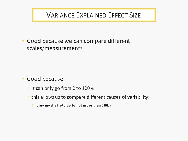
VARIANCE EXPLAINED EFFECT SIZE • Good because we can compare different scales/measurements • Good because ‣ it can only go from 0 to 100% ‣ this allows us to compare different causes of variability: • they must all add up to not more than 100%

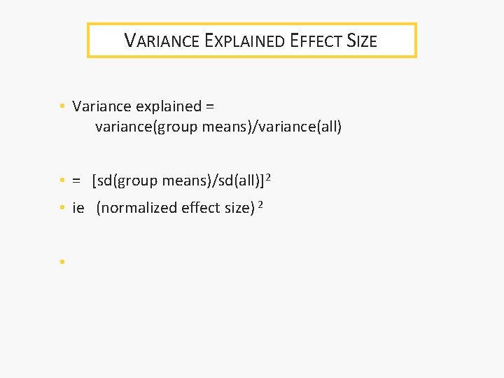
VARIANCE EXPLAINED EFFECT SIZE • Variance explained = variance(group means)/variance(all) • = [sd(group means)/sd(all)]2 • ie (normalized effect size) 2 •

EFFECT SIZE • Effect size = how strong the relationship is • 4 ways ‣ Natural ‣ Standardized ‣ Normalized ‣ Variance explained

Statistical Inference Type I errors Type II errors POWER ANALYSIS Power Analysis Prospective Power Analysis Retrospective Power Analysis

SAMPLE SIZE &INFERENCE • After we have done a study the p-value for a sample depends on: ‣ sample effect size ‣ sample size • Before we do a study the p-value we can expect to get depends on: ‣ population effect size ‣ sample size

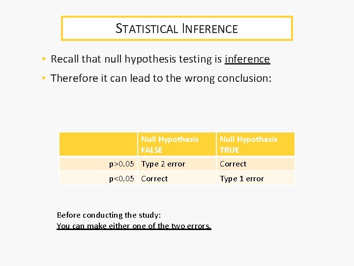
STATISTICAL INFERENCE • Recall that null hypothesis testing is inference • Therefore it can lead to the wrong conclusion: Null Hypothesis FALSE Null Hypothesis TRUE p>0. 05 Type 2 error Correct p<0. 05 Correct Type 1 error Before conducting the study: You can make either one of the two errors.

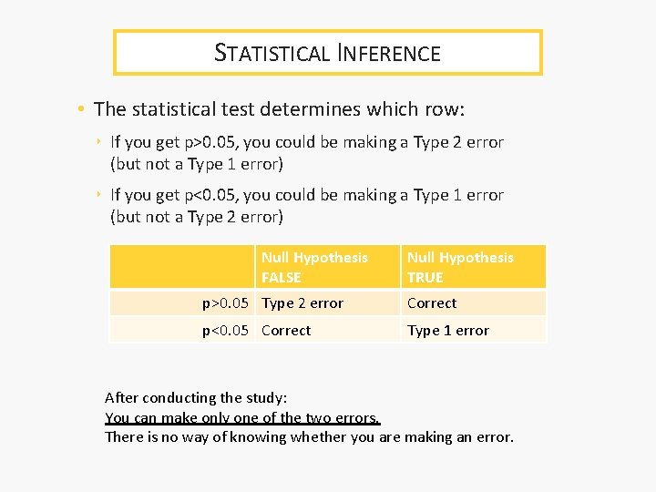
STATISTICAL INFERENCE • The statistical test determines which row: ‣ If you get p>0. 05, you could be making a Type 2 error (but not a Type 1 error) ‣ If you get p<0. 05, you could be making a Type 1 error (but not a Type 2 error) Null Hypothesis FALSE Null Hypothesis TRUE p>0. 05 Type 2 error Correct p<0. 05 Correct Type 1 error After conducting the study: You can make only one of the two errors. There is no way of knowing whether you are making an error.

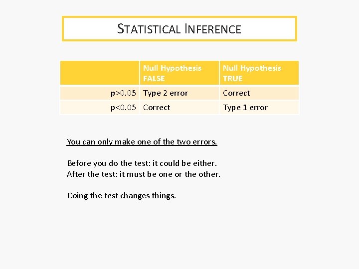
STATISTICAL INFERENCE Null Hypothesis FALSE Null Hypothesis TRUE p>0. 05 Type 2 error Correct p<0. 05 Correct Type 1 error You can only make one of the two errors. Before you do the test: it could be either. After the test: it must be one or the other. Doing the test changes things.

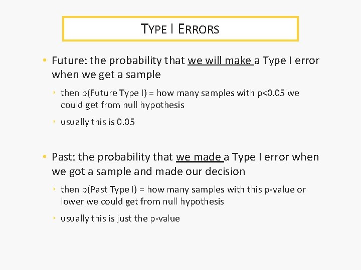
TYPE I ERRORS • Type I error concerns: ‣ future: the probability that we will make a Type I error when we get a sample ‣ past: the probability that we made a Type I error when we got a sample and made our decision

TYPE I ERRORS • Future: the probability that we will make a Type I error when we get a sample ‣ then p(Future Type I) = how many samples with p<0. 05 we could get from null hypothesis ‣ usually this is 0. 05 • Past: the probability that we made a Type I error when we got a sample and made our decision ‣ then p(Past Type I) = how many samples with this p-value or lower we could get from null hypothesis ‣ usually this is just the p-value

TYPE II ERRORS • Type II error concerns: ‣ future: the probability that we will make a Type II error when we get a sample ‣ past: the probability that we made a Type II error when we got a sample and made our decision

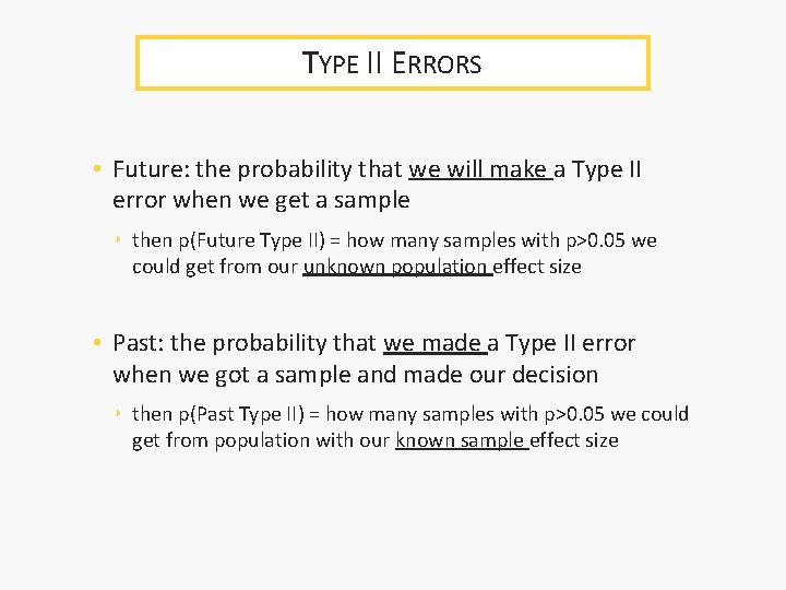
TYPE II ERRORS • Future: the probability that we will make a Type II error when we get a sample ‣ then p(Future Type II) = how many samples with p>0. 05 we could get from our unknown population effect size • Past: the probability that we made a Type II error when we got a sample and made our decision ‣ then p(Past Type II) = how many samples with p>0. 05 we could get from population with our known sample effect size

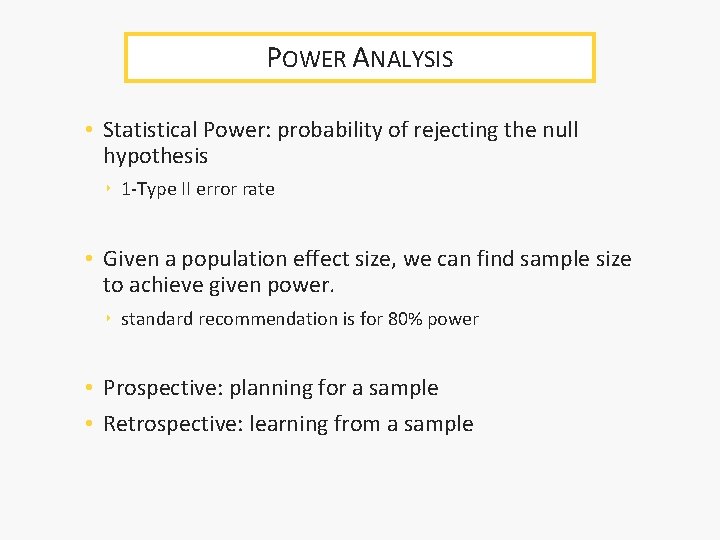
POWER ANALYSIS • Statistical Power: probability of rejecting the null hypothesis ‣ 1 -Type II error rate • Given a population effect size, we can find sample size to achieve given power. ‣ standard recommendation is for 80% power • Prospective: planning for a sample • Retrospective: learning from a sample

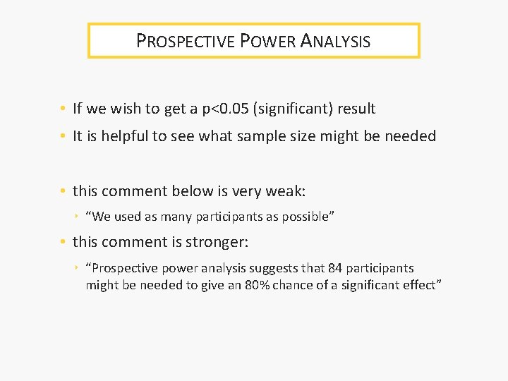
PROSPECTIVE POWER ANALYSIS • If we wish to get a p<0. 05 (significant) result • It is helpful to see what sample size might be needed • this comment below is very weak: ‣ “We used as many participants as possible” • this comment is stronger: ‣ “Prospective power analysis suggests that 84 participants might be needed to give an 80% chance of a significant effect”

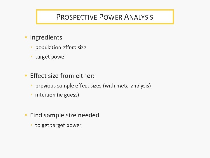
PROSPECTIVE POWER ANALYSIS • Ingredients ‣ population effect size ‣ target power • Effect size from either: ‣ previous sample effect sizes (with meta-analysis) ‣ intuition (ie guess) • Find sample size needed ‣ to get target power

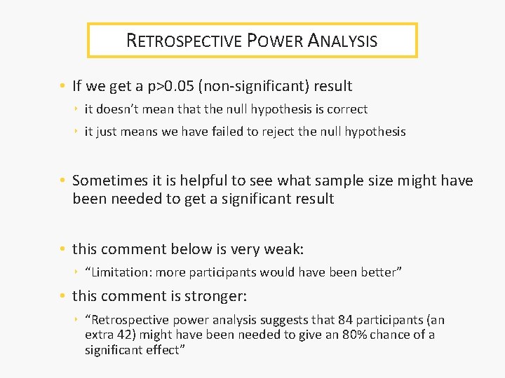
RETROSPECTIVE POWER ANALYSIS • If we get a p>0. 05 (non-significant) result ‣ it doesn’t mean that the null hypothesis is correct ‣ it just means we have failed to reject the null hypothesis • Sometimes it is helpful to see what sample size might have been needed to get a significant result • this comment below is very weak: ‣ “Limitation: more participants would have been better” • this comment is stronger: ‣ “Retrospective power analysis suggests that 84 participants (an extra 42) might have been needed to give an 80% chance of a significant effect”

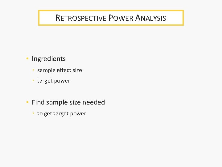
RETROSPECTIVE POWER ANALYSIS • Ingredients ‣ sample effect size ‣ target power • Find sample size needed ‣ to get target power

POWER ANALYSIS • Note the fundamental limitation of this: ‣ whichever sample effect size we use ‣ it is uncertain