Effect Modification Interaction Gl Ergr RESCAPMed Epi course


 Effect modifier - useful information (2) Confounding factor - bias")


 Disease (lung cancer) Factor B (smoking) Effect modifier =")
 and lung cancer (Ca) Case-control study, unstratified data As Yes No Total")

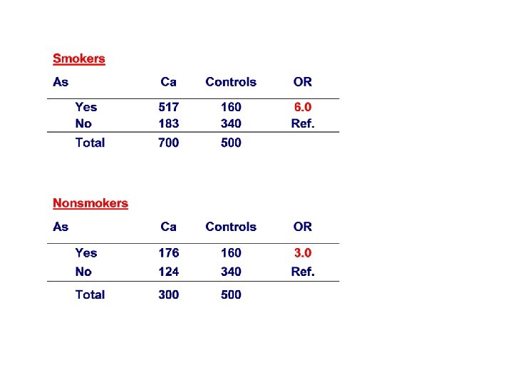
, smoking and lung cancer (Ca) As Smoking Cases Controls OR Yes 517")


 Diarrhea Controls")


 interaction Hypothetical example of")
 interaction Hypothetical example of presence")


- Slides: 47
Effect Modification -Interaction Gül Ergör RESCAP-Med Epi course, 22 -26 Sept 2014 Çeşme-Izmir
Should I believe my measurement? Exposure Outcome RR = 4 True association causal non-causal Chance? Bias? Confounding?
Exposure Outcome Third variable
Two main complications (1) Effect modifier - useful information (2) Confounding factor - bias
To analyse effect modification To eliminate confounding Solution = stratification stratified analysis Create strata according to categories inside the range of values taken by third variable
Effect modifier Variation in the magnitude of measure of effect across levels of a third variable. Happens when RR or OR is different between strata (subgroups of population)
Effect modifier To identify a subgroup with a lower or higher risk ratio To target public health action To study interaction between risk factors
Effect modification Factor A (asbestos) Disease (lung cancer) Factor B (smoking) Effect modifier = Interaction 8
Asbestos (As) and lung cancer (Ca) Case-control study, unstratified data As Yes No Total Ca Controls 693 307 320 680 1000 OR 4. 8 Ref.
Asbestos Lung cancer Smoking
Asbestos (As), smoking and lung cancer (Ca) As Smoking Cases Controls OR Yes 517 160 8. 9 Yes No 176 160 3. 0 No Yes 183 340 1. 5 No No 124 340 Ref. 1. 5 * 3. 0 < 8. 9 1. 5 * 3. 0 * interaction=8. 9
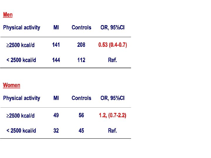
Physical activity and MI
Physical activity Infarction Gender
Any statistical test to help us? Breslow-Day Woolf test Test for trends: Chi square ti y m o H g o e n e
How to conduct a stratified analysis? Crude analysis Stratified analysis 1. 2. 3. Do stratum-specific estimates look different? 95% CI of OR/RR do NOT overlap? Is the Test of Homogeneity significant? NO Check for confounding (compare crude RR/OR with MH RR/OR) YES EFFECT MODIFICATION (Report estimates by stratum) 17
Stratified analysis: Effect Modification
Death from diarrhea according to breast feeding, Brazil, 1980 s (Crude analysis) Diarrhea Controls OR (95% CI) No breast feeding 120 136 3. 6 (2. 4 -5. 5) Breast feeding 50 204 Ref
No breast feeding Diarhoea Age
Death from diarrhea according to breast feeding, Brazil, 1980 s Infants < 1 month of age Cases Controls OR (95% CI) No breast feeding 10 3 32 (6 -203) Breast feeding 7 68 Cases Controls OR (95% CI) No breast feeding 110 133 2. 6 (1. 7 -4. 1) Breast feeding 43 136 Ref Infants ≥ 1 month of age Woolf test (test of homogeneity): p=0. 03
Examples of stratified analysis
Effect modifier Belongs to nature Different effects in different strata Simple Useful Increases knowledge of biological mechanism Allows targeting of PH action Confounding factor Belongs to study Weighted RR different from crude RR Distortion of effect Creates confusion in data Prevent (protocol) Control (analysis)
Analyzing a third factor
How to conduct a stratified analysis Perform crude analysis Measure the strength of association List potential effect modifiers and confounders Stratify data according to potential modifiers or confounders Check for effect modification If effect modification present, show the data by stratum If no effect modification present, check for confounding If confounding, show adjusted data If no confounding, show crude data
How to define the strata? • Strata defined according to third variable: – ‘Usual’ confounders (e. g. age, sex, socio-economic status) – Any other suspected confounder, effect modifier or additional risk factor – Stratum of public health interest • For two risk factors: – stratify on one to study the effect of the second on outcome • Two or more exposure categories: – each is a stratum • Residual confounding ? 26
Logical order of data analysis How to deal with multiple risk factors: Crude analysis Multivariable analysis 1. stratified analysis 2. modelling linear regression logistic regression
Multivariate analysis • Mathematical model • Simultaneous adjustment of all confounding and risk factors • Can address effect modification
Advantages & Disadvantages of Stratified Analysis • Advantages – straightforward to implement and comprehend – easy way to evaluate interaction • Disadvantages – only one exposure-disease association at a time – requires continuous variables to be grouped • Loss of information; possible “residual confounding” – deteriorates with multiple confounders • e. g. suppose 4 confounders with 3 levels – 3 x 3 x 3 x 3=81 strata needed – unless huge sample, many cells have “ 0”’ and strata have undefined effect measures 29
Interaction: Two definitions of the same phenomenon • When the effect of factor A on the probability of the outcome Y differs according to the presence of Z (and viceversa) • When the observed joint effect of (at least) factors A and Z on the probability of the outcome Y is different from that expected on the basis of the independent effects of A and Z
Interaction Individual effects A Expected joint effect A Observed joint effect Z Z A+Z No interaction Observed joint effect A+Z +I Synergism Observed joint effect A+Z -I Antagonism
Interaction Individual effects A Expected joint effect A Observed joint effect Z Z A+Z No interaction Observed joint effect A+Z +I Synergism Observed joint effect A+Z -I Antagonism
Interaction Individual effects A Expected joint effect A Observed joint effect Z Z A+Z No interaction Observed joint effect A+Z +I Synergism Observed joint effect A+Z -I Antagonism
Interaction Individual effects A Expected joint effect A Observed joint effect Z Z A+Z No interaction Observed joint effect A+Z Synergism Observed joint effect A+Z -I Antagonism
Interaction Individual effects A Expected joint effect A Observed joint effect Z Z A+Z No interaction Observed joint effect A+Z Synergism +I
Interaction Individual effects A Expected joint effect A Observed joint effect Z Z A+Z No interaction Observed joint effect A+Z Synergism Observed joint effect A+Z Antagonism +I
Interaction Individual effects A Expected joint effect A Observed joint effect Z Z A+Z No interaction Observed joint effect A+Z +I Synergism Observed joint effect A+Z Antagonism -I
Two strategies to evaluate interaction based on different, but equivalent definitions: • Effect modification (homogeneity/heterogeneity of effects) • Comparison between joint expected and joint observed effects The two definitions and strategies are completely equivalent. It is impossible to conclude that there is (or there is not) interaction using one strategy, and reach the opposite conclusion using the other strategy! Thus, when there is effect modification, the joint observed and the joint expected effects will be different.
First strategy to assess interaction: Effect Modification ADDITIVE (attributable risk) interaction Hypothetical example of presence of additive interaction Z A Incidence rate (%) No No 5. 0 Yes 10. 0 No 10. 0 Yes 30. 0 Yes ARexp to A (%) 5. 0 20. 0 Conclude: Because AR’s associated with A are modified by exposure to Z, additive interaction is present.
First strategy to assess interaction: Effect Modification MULTIPLICATIVE (ratio-based) interaction Hypothetical example of presence of multiplicative interaction Z A Incidence rate (%) No No 10. 0 Yes 20. 0 No 25. 0 Yes 125. 0 Yes RRA 2. 0 5. 0 Conclude: Because RR’s associated with A are modified by exposure to Z, multiplicative interaction is present.
Two strategies to evaluate interaction based on different, but equivalent definitions: • Effect modification (homogeneity/heterogeneity of effects) • Comparison between joint expected and joint observed effects
Second strategy to assess interaction: comparison of joint expected and joint observed effects Additive interaction Expected 5. 0 25. 0 10. 0 Joint observed AR = 25% Joint expected AR = ARA+Z- + ARA-Z+= 10% Conclude: Because the observed joint AR is different from that expected by adding the individual AR’s, additive interaction is present (that is, the same conclusion as when looking at the stratified AR’s)
Second strategy to assess interaction: comparison of joint expected and joint observed effects Multiplicative interaction 2. 0 2. 5 12. 5 5. 0 Joint observed RRA+Z+ = 12. 5 Joint expected RRA+Z+ = RRA+Z- × RRA-Z+= 2. 0 × 2. 5 = 5. 0 Conclude: Because the observed joint RR is different from that expected by multiplying the individual RR’s, there is multiplicative interaction (that is, the same conclusion as when looking at the stratified RR’s)
Further issues for discussion • Quantitative vs. qualitative interaction
Odds Ratios for the association among isolated clubfoot, maternal smoking, and a family history of clubfoot, Atlanta, Georgia, 1968 -80 Family history of clubfoot Maternal smoking Yes No Cases Controls Yes 14 7 No 11 20 Yes 118 859 No 203 2, 143 Stratified ORmaternal smk 3. 64 1. 45 Honein et al. Family history, maternal smoking, and clubfoot: an indication of geneenvironment interaction. Am J Epidemiol 2000; 152: 658 -65. Quantitative Interaction: Both ORs are in the same direction(>1. 0), but they are heterogeneous (different)
Reproductive Health Study, retrospective study of 1, 430 non-contraceptive parous women, Fishkill, NY, Burlington, VT, 1989 -90. Smoking Caffeine No. pregnancies Delayed conception* ORcaffeine No No 575 47 1. 0 301+mg/d 90 17 2. 6 No 76 15 1. 0 301+mg/d 83 11 0. 6 Yes CI 1. 4, 5. 0 0. 3, 1. 4 (Modified from: Stanton CK, Gray RH. Am J Epidemiol 1995; 142: 1322 -9) Qualitative Interaction: Odds ratios are not only different: they have different directions (>1, and <1). Smoking modifies the effect of caffeine on delayed conception in a qualitative manner.
Conclusion • If heterogeneity is present… is there interaction? – – • What is the magnitude of the difference? (p-value? ) Is it qualitative or just quantitative? If quantitative, is it additive or multiplicative? Is it biologically plausible? If we conclude that there is interaction, what should we do? – Report the stratified measures of association … The interaction may be the most important finding of the study!