EEE 4084 F Digital Systems Lecture 25 Design

EEE 4084 F Digital Systems Lecture 25: Design of Parallel Programs / T R PA Heterogeneous Computing Solutions 4 1/ Presented by: Simon Winberg

Comments concerning the title for this set of slides* Previously this aspect was referred to as “Designing Parallel Programmes” in this slides series. However I think this is somewhat restrictive; while you could consider the combination of HDL and software that runs on a heterogeneous computer as a ‘program’, I tend to think the term is too specific towards software. So I’m referring to the concept more as ‘design of heterogeneous computing solutions’. * S. Winberg See refs on last slide

Introduction These steps to designing parallel computers are pertinent to large and small scale projects. While watching these slides you can keep in mind how the topics covered could relate to your future YODA (Your Own Digital Accelerator) team project. Essentially the plan with these lectures are integrating all the pieces together into a functional HPEC system.

Lecture Overview Steps in designing parallel solutions Some of these aspects have been Step 1: understanding the problem Step 2: partitioning Step 3: decomposition & granularity

Thinking ahead, towards… Design Some Review of these slides are of course relevant when considering what you are going to be reporting on during your Design Review But NOTE: the design review assignment specifications need to be focused on when you are doing the design review (bring along some visual aid / resources to show) YODA You ‘mini conference’ can reflect briefly during your group’s presentation on aspects of what the problem is, sub-problems, partitioning methods etc.

Understanding the Problem EEE 4084 F

Steps in Designing Parallel Programs …

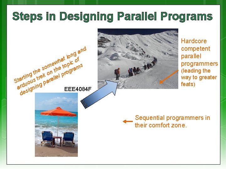
Steps in Designing Parallel Programs and g on f l t a wh pic o e om he to rams s t e h n og t r o p g rtin s trek rallel a t S uou pa g d ar ignin EEE 4084 F s e d Hardcore competent parallel programmers (leading the way to greater feats) Sequential programmers in their comfort zone.

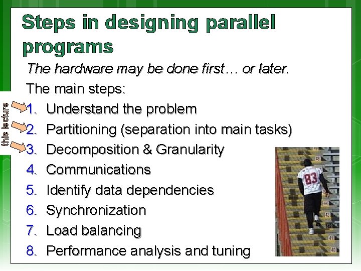
this lecture Steps in designing parallel programs … The hardware may be done first… or later. The main steps: 1. Understand the problem 2. Partitioning (separation into main tasks) 3. Decomposition & Granularity 4. Communications 5. Identify data dependencies 6. Synchronization 7. Load balancing 8. Performance analysis and tuning

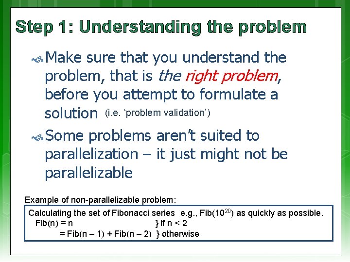
Step 1: Understanding the problem Make sure that you understand the problem, that is the right problem, before you attempt to formulate a solution (i. e. ‘problem validation’) Some problems aren’t suited to parallelization – it just might not be parallelizable Example of non-parallelizable problem: Calculating the set of Fibonacci series e. g. , Fib(1020) as quickly as possible. Fib(n) = n } if n < 2 = Fib(n – 1) + Fib(n – 2) } otherwise

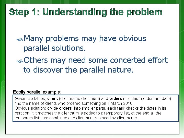
Step 1: Understanding the problem Many problems may have obvious parallel solutions. Others may need some concerted effort to discover the parallel nature. Easily parallel example: Given two tables, client (clientname, clientnum) and orders (clientnum, ordernum, date) find the name of clients who ordered something on 1 March 2010. Obvious solution: divide orders into smaller parts, each task checks the dates in its partition, it it matches the clientnum is added to a temporary list, at the end all the temporary lists are combined and clientnum replaced by clientname.

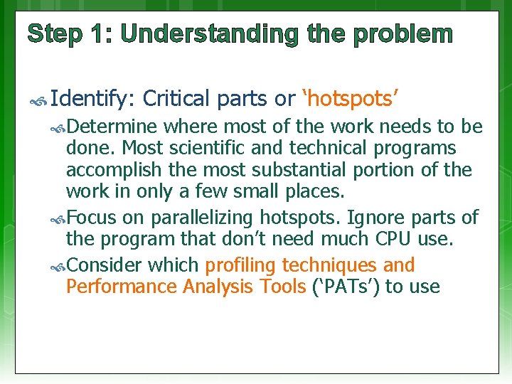
Step 1: Understanding the problem Identify: Critical parts or ‘hotspots’ Determine where most of the work needs to be done. Most scientific and technical programs accomplish the most substantial portion of the work in only a few small places. Focus on parallelizing hotspots. Ignore parts of the program that don’t need much CPU use. Consider which profiling techniques and Performance Analysis Tools (‘PATs’) to use

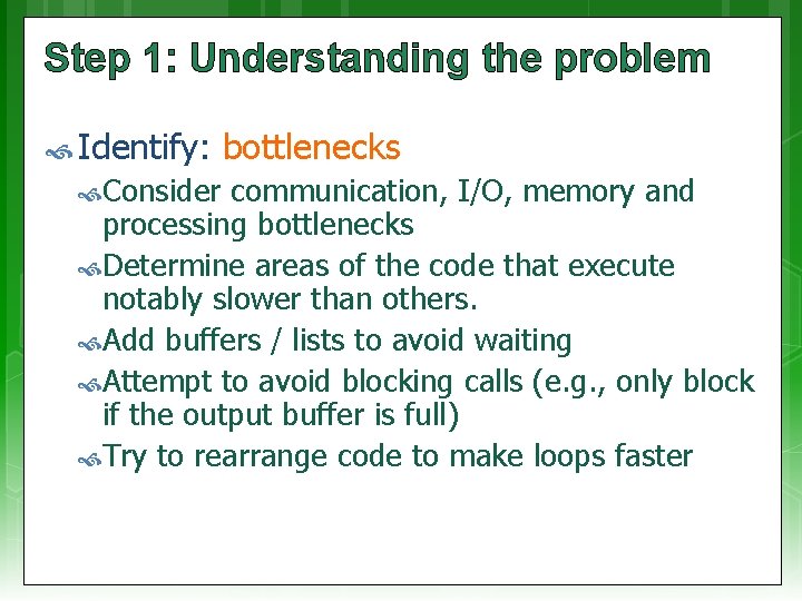
Step 1: Understanding the problem Identify: Consider bottlenecks communication, I/O, memory and processing bottlenecks Determine areas of the code that execute notably slower than others. Add buffers / lists to avoid waiting Attempt to avoid blocking calls (e. g. , only block if the output buffer is full) Try to rearrange code to make loops faster

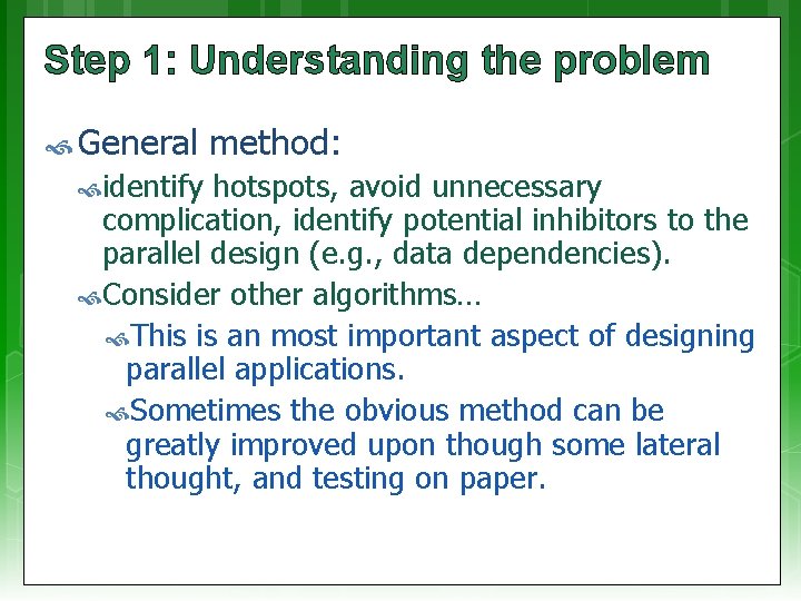
Step 1: Understanding the problem General identify method: hotspots, avoid unnecessary complication, identify potential inhibitors to the parallel design (e. g. , data dependencies). Consider other algorithms… This is an most important aspect of designing parallel applications. Sometimes the obvious method can be greatly improved upon though some lateral thought, and testing on paper.

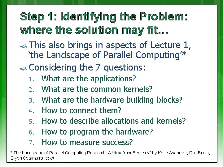
Step 1: Identifying the Problem: where the solution may fit… This also brings in aspects of Lecture 1, ‘the Landscape of Parallel Computing’* Considering the 7 questions: 1. 2. 3. 4. 5. 6. 7. What are the applications? What are the common kernels? What are the hardware building blocks? How to connect them? How to describe allocations and kernels? How to program the hardware? How to measure success? * The Landscape of Parallel Computing Research: A View from Berkeley” by Krste Asanovic, Ras Bodik, Bryan Catanzaro, et al.

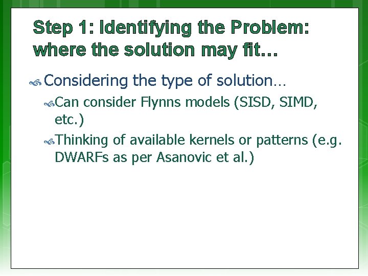
Step 1: Identifying the Problem: where the solution may fit… Considering Can the type of solution… consider Flynns models (SISD, SIMD, etc. ) Thinking of available kernels or patterns (e. g. DWARFs as per Asanovic et al. )

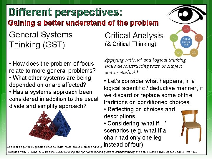
Different perspectives: Gaining a better understand of the problem General Systems Thinking (GST) • How does the problem of focus relate to more general problems? • What other systems are being depended on or are affected? • Has a systems approach been considered in addition to the usual divide and simplify approach? See last page for suggested sites to learn more about critical analysis Critical Analysis (& Critical Thinking) Applying rational and logical thinking while deconstructing texts or subject matter studied. * • Let’s consider what happens, in a logical scientific / deductive manner, if we discard or replace some of the traditions or ‘conditioned choices’. • Reflecting on choices and descriptions • Considering ‘what if…’ scenarios (e. g. what if a chair had only one leg instead of four) * Adapted from: Browne, M & Keeley, S 2001, Asking the right questions: a guide to critical thinking, 6 th edn, Prentice-Hall, Upper Saddle River, N. J.

Video Clip: Systems Thinking This is a suggested video clip to view for gaining an insight into what Systems Thinking is about. You. Tube clip: Systems thinking an introduction. mp 4

Step 2: Partitioning partitioning This The Problem step involves breaking the problem into separate chunks of work, which can then be implemented as multiple distributed tasks. Two typical methods to partition computation among parallel tasks: 1. 2. Functional decomposition or Domain decomposition

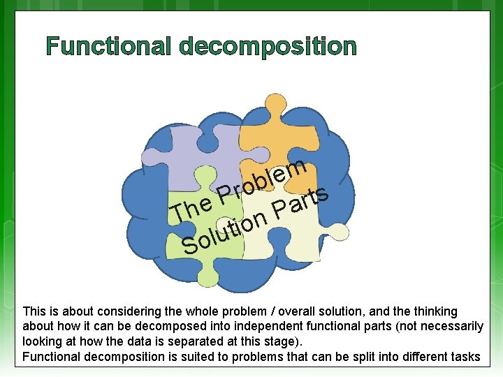
Functional decomposition m e l b o r s P t r e a h P T n o i t u l So This is about considering the whole problem / overall solution, and the thinking about how it can be decomposed into independent functional parts (not necessarily looking at how the data is separated at this stage). Functional decomposition is suited to problems that can be split into different tasks

Functional decomposition Functional Step 2: Partitioning decomposition focuses on the computation to be done, rather than the way data is separated and manipulated by tasks. The problem is decomposed into tasks according to the work that must be done. Each task performs a portion of the overall work. Tends to be closer to message passing and MIMD systems

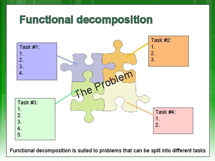
Functional decomposition Task #2: 1. 2. 3. Task #1: 1. 2. 3. 4. r P he Task #3: 1. 2. 3. 4. 5. m e l ob T Task #4: 1. 2. Functional decomposition is suited to problems that can be split into different tasks

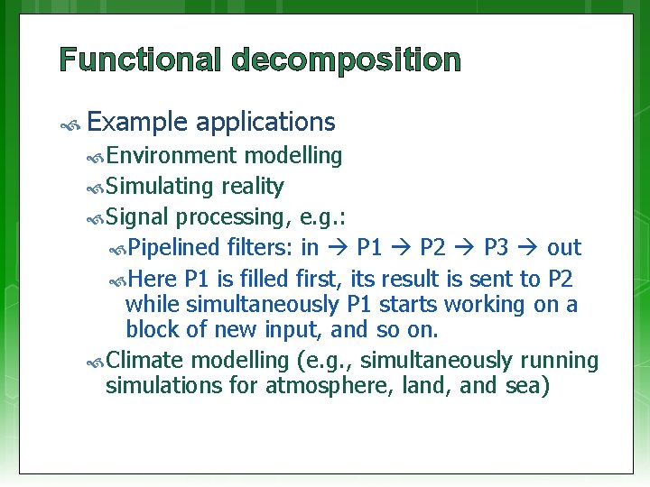
Functional decomposition Example applications Environment modelling Simulating reality Signal processing, e. g. : Pipelined filters: in P 1 P 2 P 3 out Here P 1 is filled first, its result is sent to P 2 while simultaneously P 1 starts working on a block of new input, and so on. Climate modelling (e. g. , simultaneously running simulations for atmosphere, land, and sea)

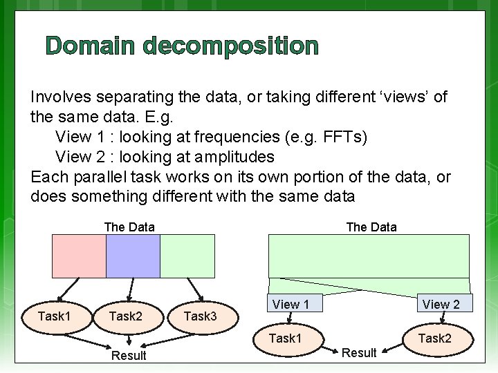
Domain decomposition Involves separating the data, or taking different ‘views’ of the same data. E. g. View 1 : looking at frequencies (e. g. FFTs) View 2 : looking at amplitudes Each parallel task works on its own portion of the data, or does something different with the same data The Data Task 1 Task 2 The Data Task 3 View 1 View 2 Task 1 Result Task 2 Result

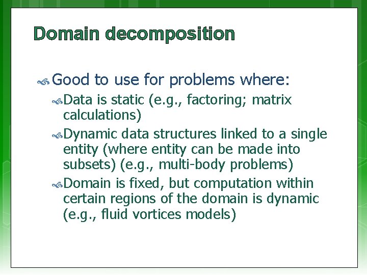
Domain decomposition Good Data to use for problems where: is static (e. g. , factoring; matrix calculations) Dynamic data structures linked to a single entity (where entity can be made into subsets) (e. g. , multi-body problems) Domain is fixed, but computation within certain regions of the domain is dynamic (e. g. , fluid vortices models)

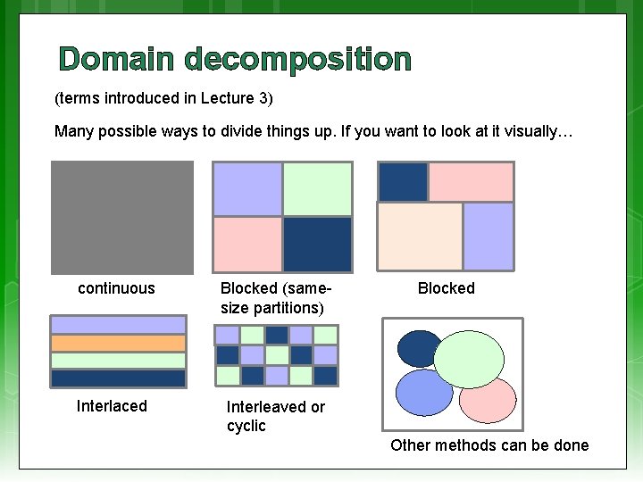
Domain decomposition (terms introduced in Lecture 3) Many possible ways to divide things up. If you want to look at it visually… continuous Blocked (samesize partitions) Interlaced Interleaved or cyclic Blocked Other methods can be done

Step 3: Decomposition and Granularity EEE 4084 F

Step 3: Decomposition and Granularity Decomposition – how the problem can be divided up; looked at earlier: Functional decomposition Domain (or data) decomposition Granularity How big or small are the parts that the problem has been decomposed into? How interrelated are the sub-tasks This was introduced this in Lecture 5

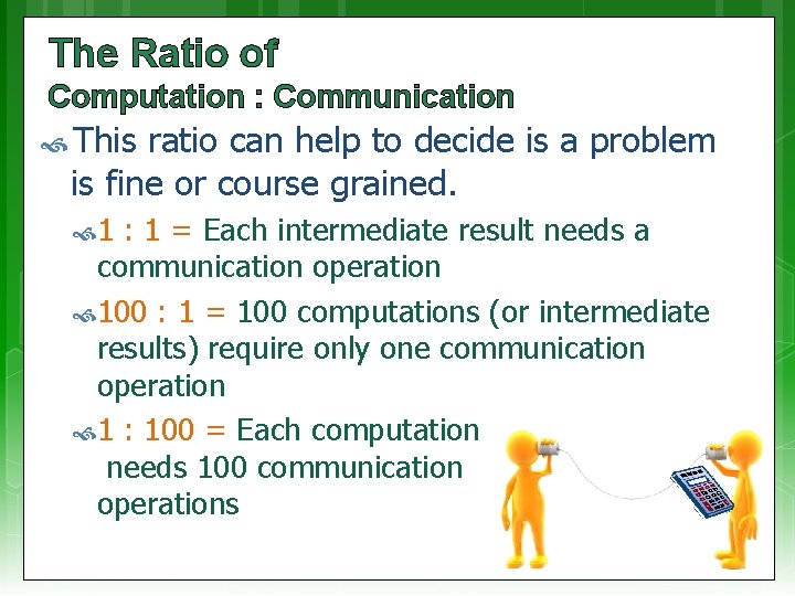
The Ratio of Computation : Communication This ratio can help to decide is a problem is fine or course grained. 1 : 1 = Each intermediate result needs a communication operation 100 : 1 = 100 computations (or intermediate results) require only one communication operation 1 : 100 = Each computation needs 100 communication operations

Granularity Fine Grained: One part / sub-process requires a great deal of communication with other parts to complete its work relative to the amount of computing it does (the ratio computation : communication is low, approaching 1: 1) course grained …

Granularity Fine Grained: One part / sub-process requires a great deal of communication with other parts to complete its work relative to the amount of computing it does (the ratio computation : communication is low, approaching 1: 1) Course A Grained: coarse-grained parallel task is largely independent of other tasks. But still requires some communication to complete its part. The computation : communication ratio is high (say around 100: 1).

Granularity Fine Grained: One part / sub-process requires a great deal of communication with other parts to complete its work relative to the amount of computing it does (the ratio computation : communication is low, approaching 1: 1) Course Grained: A coarse-grained parallel task is largely independent of other tasks. But still requires some communication to complete its part. The computation : communication ratio is high (say around 100: 1). Embarrassingly So Parallel: course that there’s no or very little interrelation between parts/sub-processes

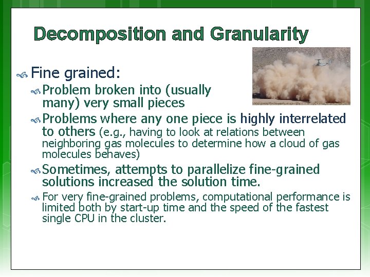
Decomposition and Granularity Fine grained: Problem broken into (usually many) very small pieces Problems where any one piece is highly interrelated to others (e. g. , having to look at relations between neighboring gas molecules to determine how a cloud of gas molecules behaves) Sometimes, attempts to parallelize fine-grained solutions increased the solution time. For very fine-grained problems, computational performance is limited both by start-up time and the speed of the fastest single CPU in the cluster.

Decomposition and Granularity Course grained: Breaking the problems into larger pieces Usually, low level of interrelations (e. g. , can separate into parts whose elements are unrelated to other parts) These solutions are generally easier to parallelize than finegrained, and Usually, parallelization of these problems provides significant benefits. Ideally, the problem is found to be “embarrassingly parallel” (this can of course also be the case for fine grained solutions)

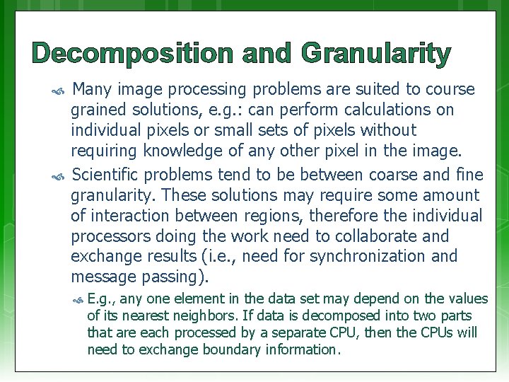
Decomposition and Granularity Many image processing problems are suited to course grained solutions, e. g. : can perform calculations on individual pixels or small sets of pixels without requiring knowledge of any other pixel in the image. Scientific problems tend to be between coarse and fine granularity. These solutions may require some amount of interaction between regions, therefore the individual processors doing the work need to collaborate and exchange results (i. e. , need for synchronization and message passing). E. g. , any one element in the data set may depend on the values of its nearest neighbors. If data is decomposed into two parts that are each processed by a separate CPU, then the CPUs will need to exchange boundary information.

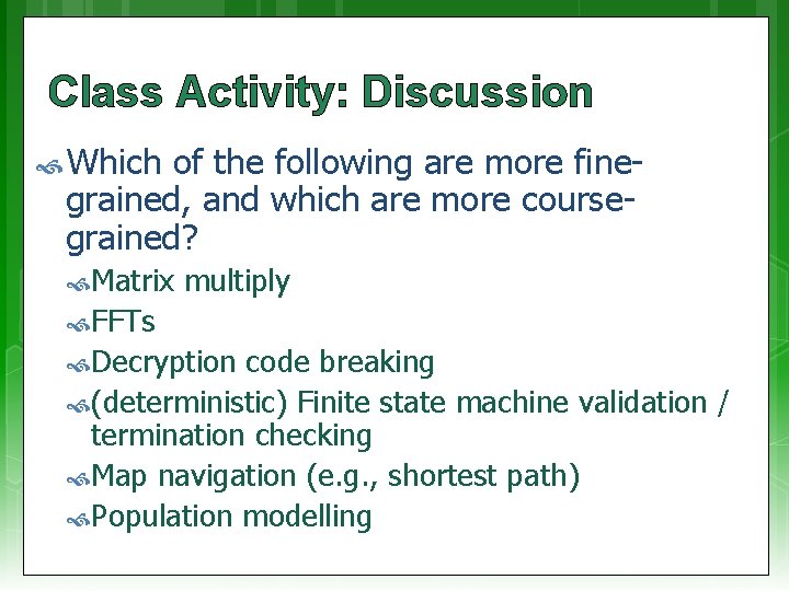
Class Activity: Discussion Which of the following are more finegrained, and which are more coursegrained? Matrix multiply FFTs Decryption code breaking (deterministic) Finite state machine validation / termination checking Map navigation (e. g. , shortest path) Population modelling

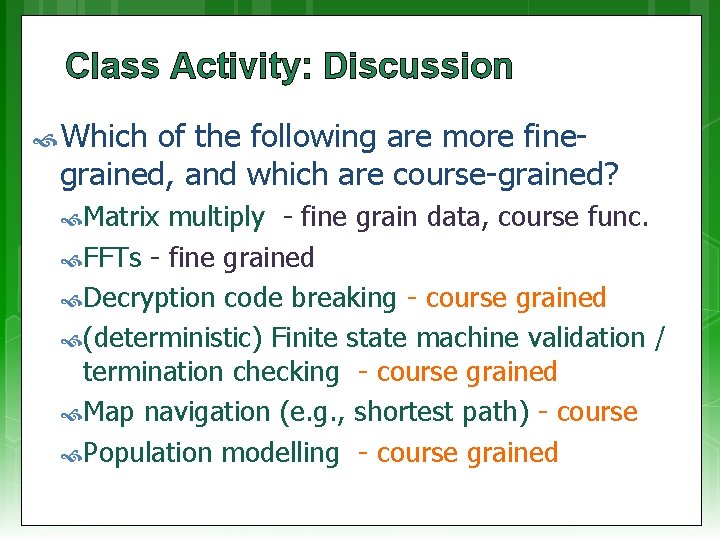
Class Activity: Discussion Which of the following are more finegrained, and which are course-grained? Matrix multiply - fine grain data, course func. FFTs - fine grained Decryption code breaking - course grained (deterministic) Finite state machine validation / termination checking - course grained Map navigation (e. g. , shortest path) - course Population modelling - course grained

Next lecture Continuation of the steps: Communications Identify data dependencies Synchronization Load balancing Performance analysis and tuning

Further Reading / Refs Suggestions for further reading, slides partially based / general principles elaborated in: • https: //computing. llnl. gov/tutorials/parallel_comp/ • http: //www 2. physics. uiowa. edu/~ghowes/teach/ihpc 12/lec/ihpc 12 Lec_Desig n. HPC 12. pdf Some resources related to systems thinking: • https: //www. youtube. com/watch? v=lhb. LNBqh. Qkc • https: //www. youtube. com/watch? v=AP 7 h. Mdn. Nr. H 4 Some resources related to critical analysis and critical thinking: An easy introduction to critical analysis: • http: //www. deakin. edu. au/current-students/study-support/studyskills/handouts/critical-analysis. php An online quiz and learning tool for understanding critical thinking: • http: //unilearning. uow. edu. au/critical/1 a. html