EECS 373 Design of MicroprocessorBased Systems Prabal Dutta

EECS 373 Design of Microprocessor-Based Systems Prabal Dutta University of Michigan Sampling, ADCs, and DACs Some slides adapted from Mark Brehob, Jonathan Hui & Steve Reinhardt 1

Announcements • Exam is a 7 days from today – Q&A session on Monday (10/26) during class – Practice exam/HW#5 due Friday • Group Projects – Research projects: let me know if interested – Time to find group members – Brainstorm project ideas! 2

Outline • Announcements • Sampling • ADC • DAC 3

We live in an analog world • Everything in the physical world is an analog signal – Sound, light, temperature, pressure • Need to convert into electrical signals – Transducers: converts one type of energy to another • Electro-mechanical, Photonic, Electrical, … – Examples • Microphone/speaker • Thermocouples • Accelerometers 4

Transducers convert one form of energy into another • Transducers – Allow us to convert physical phenomena to a voltage potential in a well-defined way. A transducer is a device that converts one type of energy to another. The conversion can be to/from electrical, electro-mechanical, electromagnetic, photonic, photovoltaic, or any other form of energy. While the term transducer commonly implies use as a sensor/detector, any device which converts energy can be considered a transducer. – Wikipedia. 5
 RR/(R")
Convert light to voltage with a Cd. S photocell Vsignal = (+5 V) RR/(R + RR) • Choose R = (RR at median of intended range) • Cadmium Sulfide (Cd. S) • Cheap, low current • t. RC = (R+RR)*Cl – – Typically R~50 -200 k. W C~20 p. F So, t. RC~20 -80 u. S f. RC ~ 10 -50 k. Hz Source: Forrest Brewer 6
 • Force • Acceleration – strain gauges -")
Many other common sensors (some digital) • Force • Acceleration – strain gauges - foil, conductive ink – conductive rubber – rheostatic fluids • Piezorestive (needs bridge) – piezoelectric films – capacitive force • Charge source • Sound – Microphones • Both current and charge versions – Sonar • Usually Piezoelectric • Position – microswitches – shaft encoders – gyros Source: Forrest Brewer – MEMS – Pendulum • Monitoring – Battery-level • voltage – Motor current • Stall/velocity – Temperature • Voltage/Current Source • Field – Antenna – Magnetic • Hall effect • Flux Gate • Location – Permittivity – Dielectric

Going from analog to digital • What we want Physical Phenomena Engineering Units • How we have to get there Physical Phenomena Voltage or Current Sensor Engineering Units ADC Counts ADC Software 8

Representing an analog signal digitally • How do we represent an analog signal (e. g. continuous voltage)? – As a time series of discrete values On MCU: read ADC data register (counts) periodically (Ts) Voltage (continuous) Counts (discrete) 9
 •")
Choosing the range • Fixed # of bits (e. g. 8 -bit ADC) • Span a particular input voltage range • What do the sample values represent? – Some fraction within the range of values What range to use? Range Too Big Range Too Small Ideal Range 10

Choosing the granularity • Resolution – Number of discrete values that represent a range of analog values – MSP 430: 12 -bit ADC • 4096 values • Range / 4096 = Step Larger range less info / bit • Quantization Error – How far off discrete value is from actual – ½ LSB Range / 8192 Larger range larger error 11

Choosing the sample rate • What sample rate do we need? – Too little: we can’t reconstruct the signal we care about – Too much: waste computation, energy, resources 12

Shannon-Nyquist sampling theorem • If a continuous-time signal contains no frequencies higher than , it can be completely determined by discrete samples taken at a rate: • Example: – Humans can process audio signals 20 Hz – 20 KHz – Audio CDs: sampled at 44. 1 KHz 13

Converting between voltages, ADC counts, and engineering units • Converting: ADC counts Voltage • Converting: Voltage Engineering Units 14

A note about sampling and arithmetic* • Converting values in fixed-point MCUs float vtemp = adccount/4095 * 1. 5; float tempc = (vtemp-0. 986)/0. 00355; vtemp = 0! Not what you intended, even when vtemp is a float! tempc = -277 C • Fixed point operations – Need to worry about underflow and overflow • Floating point operations – They can be costly on the node 15
")
Try it out for yourself… $ cat arithmetic. c #include <stdio. h> int main() { int adccount = 2048; float vtemp; float tempc; vtemp = adccount/4095 * 1. 5; tempc = (vtemp-0. 986)/0. 00355; printf("vtemp: %fn", vtemp); printf("tempc: %fn", tempc); } $ gcc arithmetic. c $. /a. out vtemp: 0. 000000 tempc: -277. 746490 16

Use anti-aliasing filters on ADC inputs to ensure that Shannon-Nyquist is satisfied • Aliasing – Different frequencies are indistinguishable when they are sampled. • Condition the input signal using a low-pass filter – Removes high-frequency components – (a. k. a. anti-aliasing filter) 17

Designing the anti-aliasing filter • Note • w is in radians • w = 2 pf • Exercise: Say you want the half-power point to be at 30 Hz and you have a 0. 1 μF capacitor. How big of a resistor should you use? 18

Do I really need to condition my input signal? • Short answer: Yes. • Longer answer: Yes, but sometimes it’s already done for you. – Many (most? ) ADCs have a pretty good analog filter built in. – Those filters typically have a cut-off frequency just above ½ their maximum sampling rate. • Which is great if you are using the maximum sampling rate, less useful if you are sampling at a slower rate. 19

Oversampling • One interesting trick is that you can use oversampling to help reduce the impact of quantization error. – Let’s look at an example of oversampling plus dithering to get a 1 -bit converter to do a much better job… 20
 Voltage uniformly distributed random")
Oversampling a 1 -bit ADC w/ noise & dithering (cont) Voltage uniformly distributed random noise Count “upper edge” of the box ± 250 m. V Vthresh = 500 m. V 375 m. V Vrand = 500 m. V 1 N 1 = 11 N 0 = 32 0 0 m. V Note: N 1 is the # of ADC counts that = 1 over the sampling window N 0 is the # of ADC counts that = 0 over the sampling window 21
 • • How to")
Oversampling a 1 -bit ADC w/ noise & dithering (cont) • • How to get more than 1 -bit out of a 1 -bit ADC? Add some noise to the input Do some math with the output Example – – 1 -bit ADC with 500 m. V threshold Vin = 375 m. V ADC count = 0 Add ± 250 m. V uniformly distributed random noise to Vin Now, roughly • 25% of samples (N 1) ≥ 500 m. V ADC count = 1 • 75% of samples (N 0) < 500 m. V ADC count = 0 – So, the “upper edge” of the box equals • Vthresh + N 1/(N 1+N 0) * Vrand = 0. 5 + 11/(11+32)*0. 5 = 0. 628 V – Middle of box (where our “signal” of 375 m. V sits) equals • 0. 628 V – Vrand/2 = 0. 628 V – 0. 25 = 0. 378 V – Real value is 0. 375 V, so our estimate has < 1% error! 22

Can use dithering to deal with quantization • Dithering – Quantization errors can result in large-scale patterns that don’t accurately describe the analog signal – Oversample and dither – Introduce random (white) noise to randomize the quantization error. Direct Samples Dithered Samples 23
 filter on the output •")
Lots of other issues • Might need anti-imaging (reconstruction) filter on the output • Cost, speed (, and power): • Might be able to avoid analog all together – Think PWM when dealing with motors… 24

How do ADCs and DACs work? • Many different types! • DAC – DAC #1: Voltage Divider – DAC #2: R/2 R Ladder • ADC – ADC #1: Flash – ADC #2: Single-Slope Integration – ADC #3: Successive Approximate (SAR) 25

DAC #1: Voltage Divider Vref R Din 2 2 -to-4 decoder • Fast • Size (transistors, switches)? • Accuracy? • Monotonicity? R R Vout R 26

DAC #2: R/2 R Ladder Vref 2 R R R 2 R 2 R Iout D 3 (MSB) D 2 D 1 D 0 (LSB) • Size? • Accuracy? • Monotonicity? (Consider 0111 -> 1000) 27

DAC output signal conditioning • Often use a low-pass filter • May need a unity gain op amp for drive strength 28

ADC #1: Flash Converter Vref R R R Vin + _ priority encoder 3 2 2 Dout + _ 1 Vcc 0 R 29

ADC #1: Flash Converter Example Vin = 2. 5 V Vref 4 V R 3 V R 2 V R 1 V 2. 5 + 3. 0 _3 2. 5 + 2. 0 _2 ‘H’ 2. 5 ‘H’ + 1. 0 _1 R 0 V ‘L’ Vcc ‘H’ priority encoder 3 2 1 0 2 • Resistors divide Vref, e. g. • Let Vref = 4 V • 4 equal resistors => 1 V steps • The 1 V, 2 V, and 3 V signals are fed into the negative input of three comparators • A comparator outputs a logic high (‘H’) if its positive input is greater than its negative input • For comparator #1 and #2, this is Dout indeed the case (2. 5 V > 1 V and 2. 5 0 b 10 V > 2 V, respectively), so they outputs a logic high, ‘H’ • For comp #3, (2. 5 V < 3. 0 V), so it outputs a logic low, ‘L’ • A priority encoder outputs the largest numbered input that is high (true). Since 0, 1, and 2 are all true, Dout = 0 b 10. 30

ADC #2: Single-Slope Integration Vin + _ Vcc done I C EN* n-bit counter CLK • Start: Reset counter, discharge C. • Charge C at fixed current I until Vc > Vin. How should C, I, n, and CLK (f. CLK) be related? • Final counter value is Dout. • Conversion may take several milliseconds. • Good differential linearity. • Absolute linearity depends on precision of C, I, and clock. 31
 1 Sample Multiple cycles • Requires N-cycles per sample")
ADC #3: Successive Approximation (SAR) 1 Sample Multiple cycles • Requires N-cycles per sample where N is # of bits • Goes from MSB to LSB • Not good for high-speed ADCs 32

Errors and ADCs • Figures and some text from: – Understanding analog to digital converter specifications. By Len Staller – http: //www. embedded. com/show. Article. jhtml? article. ID=60403334 • Key concept here is that the specification provides worst case values.
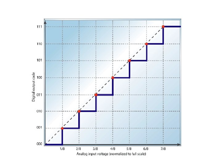
 is the deviation of an ADC's transfer function")
Integral nonlinearity The integral nonlinearity (INL) is the deviation of an ADC's transfer function from a straight line. This line is often a best-fit line among the points in the plot but can also be a line that connects the highest and lowest data points, or endpoints. INL is determined by measuring the voltage at which all code transitions occur and comparing them to the ideal. The difference between the ideal voltage levels at which code transitions occur and the actual voltage is the INL error, expressed in LSBs. INL error at any given point in an ADC's transfer function is the accumulation of all DNL errors of all previous (or lower) ADC codes, hence it's called integral nonlinearity.

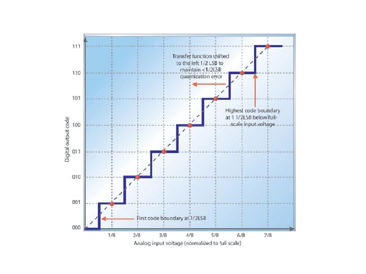
Differential nonlinearity DNL is the worst cases variation of actual step size vs. ideal step size. It’s a promise it won’t be worse than X.

Sometimes the intentional ½ LSB shift is included here!

Full-scale error is also sometimes called “gain error” full-scale error is the difference between the ideal code transition to the highest output code and the actual transition to the output code when the offset error is zero.

Errors • Once again: Errors in a specification are worst case. – So if you have an INL of ±. 25 LSB, you “know” that the device will never have more than. 25 LSB error from its ideal value. – That of course assumes you are operating within the specification • Temperature, input voltage, input current available, etc. • INL and DNL are the ones we expect you to work with – Should know what full-scale error is
- Slides: 40