EECS 274 Computer Vision Segmentation by Clustering Segmentation

EECS 274 Computer Vision Segmentation by Clustering

Segmentation and Grouping • Motivation: Obtain a compact representation from an image/motion sequence/set of tokens • Should support application • Broad theory is absent at present • Reading: FP Chapter 14, S Chapter 5 • Grouping (or clustering) – collect together tokens that “belong together” • Fitting – associate a model with tokens – issues • which model? • which token goes to which element? • how many elements in the model?

How do they assemble? Why do these tokens belong together? • because they form surfaces? • because they form the same texture?

Segmentation: examples • • Summarizing videos: shots Finding matching parts Finding people Finding buildings in satellite images Searching a collection of images Object detection Object recognition

Models problems • Forming image segments: super pixels, image regions • Fitting lines to edge points • Fitting a fundamental matrix to a set of feature points: – If the correspondence is right, there is a fundamental matrix connecting the points

Segmentation as clustering • Partitioning – Decompose into regions that have coherent color and texture – Decompose into extended blobs, consisting of regions that have coherent color, texture, and motion – Take a video sequence and decompose it into shots • Grouping – Collecting together tokens that, taken together, form a line – Collecting together tokens that seem to share a fundamental matrix • What is the appropriate representation?

General ideas • Tokens – whatever we need to group (pixels, points, surface elements, etc. ) • Top down segmentation – tokens belong together because they lie on the same object • Bottom up segmentation – tokens belong together because they are locally coherent • These two are not mutually exclusive

Grouping and gestalt • Gestalt school of psychology – Studying shape as a whole instead of just a collection of simple and curves – Grouping means the tendency of visual system to assemble components together and perceive them together Muller-Lyer illusion

Some Gestalt properties emergence reification

Figure and ground • White circle/black rectangle: which is figure (foreground) and which is ground (background)?

Basic ideas of grouping in humans • Figure-ground discrimination – grouping can be seen in terms of allocating some elements to a figure, some to ground – impoverished theory • Gestalt properties – elements in a collection of elements can have properties that result from relationships (Muller-Lyer effect) • gestalt qualitat (form quality) – A series of factors affect whether elements should be grouped together • Gestalt factors

Gestalt movement

Examples of Gestalt factors

Example

Occlusion as a cue

Grouping phenomena

Illusory contours Tokens appear to be grouped together as they provide a cue to the presence of an occluding object whose contour has no contrast

Background Subtraction • If we know what the background looks like, it is easy to identify “interesting bits” • Applications – person in an office – tracking cars on a road – surveillance • Approach: – use a moving average to estimate background image – subtract from current frame – large absolute values are interesting pixels • trick: use morphological operations to clean up pixels

Results using 80 x 60 frames (a) Average of all 120 frames. (b) thresholding. (c) results with low threshold (with missing pixels). (d) background computed using the EM-based algorithm. (e) background subtraction results (with missing pixels).

Results using 160 x 120 frames (a) Average of all 120 frames. (b) thresholding. (c) results with low threshold (with missing pixels). (d) background computed using the EM-based algorithm. (e) background subtraction results (with missing pixels).

Shot boundary detection • Find the shots in a sequence of video – shot boundaries usually result in big differences between succeeding frames – allows for objects to move within a given shot • Strategy: – compute interframe distances – declare a boundary where these are big • Possible distances – – frame differences histogram differences block comparisons edge differences • Applications: – representation for movies, or video sequences • find shot boundaries • obtain “most representative” frame – supports search

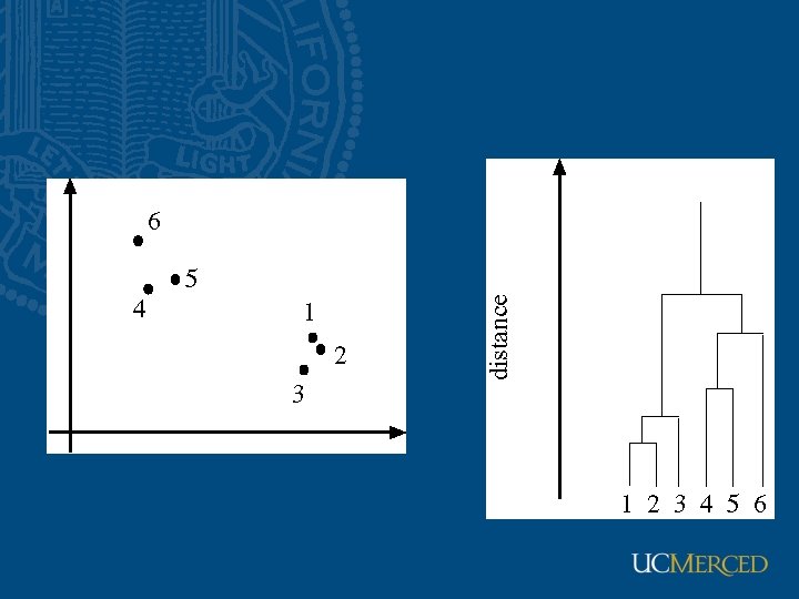
Segmentation as clustering • Cluster together (pixels, tokens, etc. ) that belong together • Agglomerative clustering – attach closest to cluster it is closest to – repeat • Divisive clustering – split cluster along best boundary – repeat • Point-Cluster distance – single-link clustering (distance between two closest elements) – complete-link clustering (maximum distance between two elements) – group-average clustering • Dendrograms (tree diagram) – yield a picture of output as clustering process continues

K-Means • Choose a fixed number of clusters • Choose cluster centers and point-cluster allocations to minimize error • can’t do this by search, because there are too many possible allocations. • Algorithm – fix cluster centers; allocate points to closest cluster – fix allocation; compute best cluster centers • x could be any set of features for which we can compute a distance (careful about scaling)

Image Clusters on intensity Clusters on color K-means clustering using intensity alone and color alone How many clusters?

Image Clusters on color K-means using color alone, 11 segments (6 kinds of vegetables)

K-means using color alone, 11 segments (not using texture or position) - segments may be disconnected and scattered

K-means using color and position, 20 segments - peppers are now separated but, cabbage is still broken up

Graph-theoretic clustering • Represent tokens using a weighted graph. – affinity matrix – similar have large weights • Cut up this graph to get connected components – with strong interior links – by cutting edges with low weights • A graph is a set of vertices V and edges E, G={V, E} • A weighted graph is one in which each edge is associated with a weight • Every graph consists of a disjoint set of connected components

Weighted graph 9 points/pixels A cut with 2 connected components 9 x 9 Weighted matrix that looks like block diagonal

(Left) a set of points (Right) affinity matrix computed with a decaying exponential distance (large values bright pixels, and small values dark pixels)

Graph cut and normalized cut sum of all the weights associated with nodes in A

Affinity Intensity Distance Texture

Scale affects affinity σ=0. 1 σ=0. 2 σ=1

Extracting a single good cluster • Simplest idea: we want a vector a giving the association between each element and a cluster • We want elements within this cluster to, on the whole, have strong affinity with one another • We could maximize • But need the constraint • Solving constrained optimization with Lagrange multiplier • This is an eigenvalue problem choose the eigenvector of A with largest eigenvalue association of element i with cluster n × affinity between i and j × association of element j and cluster n

Example eigenvector points eigenvector matrix

Clustering with eigenvectors • If we reorder the nodes, the rows and columns of A are shuffled • We expect to deal with a few clusters with large association • We could shuffle the rows and columns of M to form a matrix that is roughly block diagonal • Shuffling M simply shuffle the elements of its eigenvectors so • We can reason about the eigenvectors by working with a shuffled version of M

Eigenvectors and clusters • Eigenvectors of block-diagonal matrices consist of eigenvectors of the blocks padded with zeros • Each block has an eigenvector corresponding to a rather large eigenvalue • Expect that, if there are c significant clusters, the eigenvectors corresponding to the c largest eigenvalue

Large eigenvectors and clusters

Eigen gap and clusters σd=0. 1 σd=0. 2 σd=1

More than two segments • Two options – Recursively split each side to get a tree, continuing till the eigenvalue are too small – Use the other eigenvectors

Normalized cuts • Current criterion evaluates within cluster similarity, but not across cluster difference • Can also use Cheeger constant • Instead, we’d like to maximize the within cluster similarity compared to the across cluster difference • Write graph as V, one cluster as A and the other as B • Maximize • i. e. construct A, B such that their within cluster similarity is high compared to their association with the rest of the graph

Normalized cuts • Write a vector y whose elements are 1 if item is in A, -b if it’s in B • Write the matrix of the graph as W, and the matrix which has the row sums of W on its diagonal as D, 1 is the vector with all ones. • Criterion becomes • and we have a constraint • This is hard to do, because y’s values are quantized

Normalized cuts and spectral graph theory • Instead, solve the generalized eigenvalue problem • which gives • Now look for a quantization threshold that maximizes the criterion --i. e all components of y above that threshold go to one, all below go to -b

Using affinity based on texture and intensity. Figure from “Image and video segmentation: the normalized cut framework”, by Shi and Malik, copyright IEEE, 1998

Using spatio-temoral affinity metric. Figure from “Normalized cuts and image segmentation, ” Shi and Malik, copyright IEEE, 2000

Spectral clustering Ng, Jordan and Weiss, NIPS 01

Comparisons 8 clusters 4 clusters 3 clusters 2 clusters 3 clusters Ng, Jordan and Weiss, NIPS 01 2 clusters 3 clusters 2 clusters 8 clusters

Spectral graph theory generalized eigenvalue problem • See EECS 275 Lecture 23 for more detail • See also Laplacian eigenmap, Laplace Beltrami operator, Laplacian eigenmap, spectral clustering, graph cut, minimal-cut maximum-flow, normalized cut, random walk, heat kernel, diffusion map

More information • G. Scott and H. Longuet-Higgins, Feature grouping by relocalisation of eigenvectors of the proximity matrix, BMVC, 1990 • F. Chung, Spectral graph theory, AMS 1997 • Y. Weiss, Segmentation using eigenvectors: a unifying view, ICCV 1999 • L. Saul et al. , Spectral methods for dimensionality reduction, in Semisupervised learning, 2006 • U von Luxburg, A tutorial on spectral clustering, Statistics and Computing, 2007

Related topics • • • Watershed Multiscale segmentation Mean-shift segmentation Parsing tree/stochastic grammar Graph cut Objet cut Grab cut Random walk Energy-based method