EECS 105 Fall 2003 Lecture 1 Course Overview

EECS 105 Fall 2003, Lecture 1: Course Overview and Introduction to Phasors Prof. Niknejad Department of EECS University of California, Berkeley

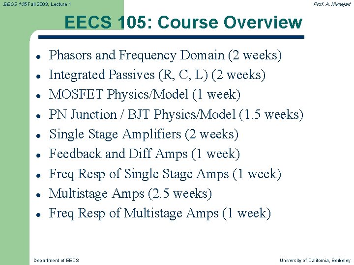
EECS 105 Fall 2003, Lecture 1 Prof. A. Niknejad EECS 105: Course Overview l l l l l Phasors and Frequency Domain (2 weeks) Integrated Passives (R, C, L) (2 weeks) MOSFET Physics/Model (1 week) PN Junction / BJT Physics/Model (1. 5 weeks) Single Stage Amplifiers (2 weeks) Feedback and Diff Amps (1 week) Freq Resp of Single Stage Amps (1 week) Multistage Amps (2. 5 weeks) Freq Resp of Multistage Amps (1 week) Department of EECS University of California, Berkeley

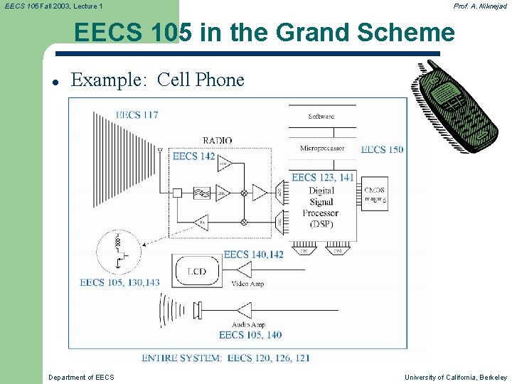
EECS 105 Fall 2003, Lecture 1 Prof. A. Niknejad EECS 105 in the Grand Scheme l Example: Cell Phone Department of EECS University of California, Berkeley

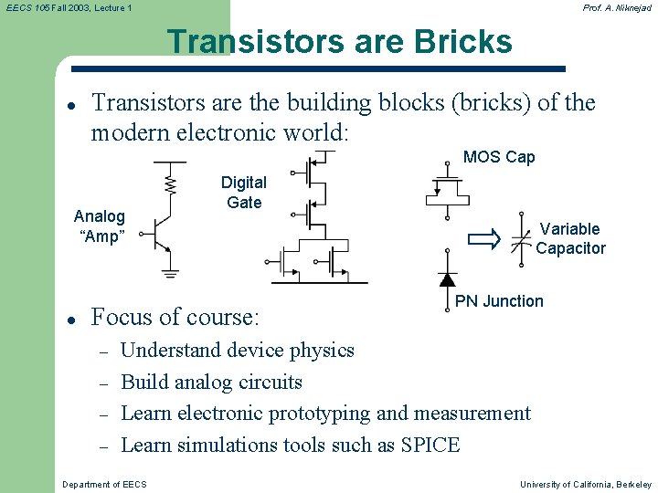
EECS 105 Fall 2003, Lecture 1 Prof. A. Niknejad Transistors are Bricks l Transistors are the building blocks (bricks) of the modern electronic world: MOS Cap Analog “Amp” l Digital Gate Focus of course: – – Variable Capacitor PN Junction Understand device physics Build analog circuits Learn electronic prototyping and measurement Learn simulations tools such as SPICE Department of EECS University of California, Berkeley

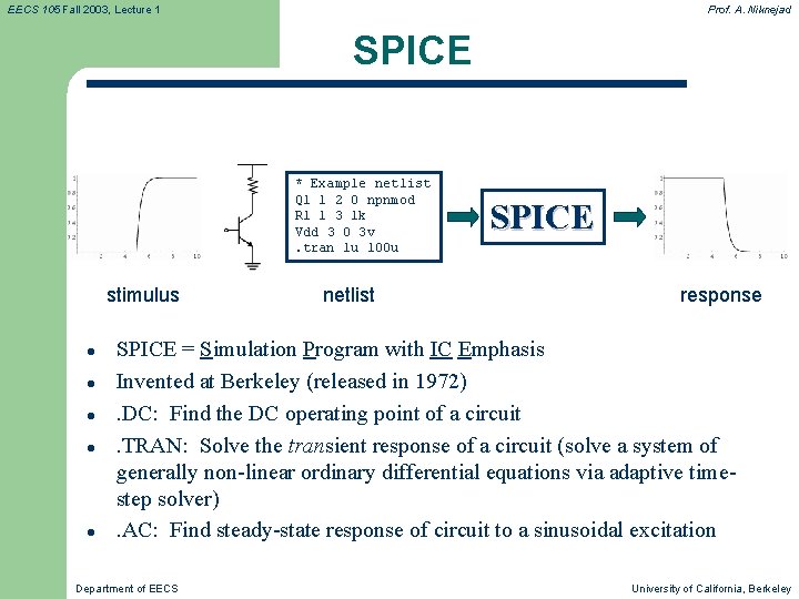
EECS 105 Fall 2003, Lecture 1 Prof. A. Niknejad SPICE * Example netlist Q 1 1 2 0 npnmod R 1 1 3 1 k Vdd 3 0 3 v. tran 1 u 100 u stimulus l l l netlist SPICE response SPICE = Simulation Program with IC Emphasis Invented at Berkeley (released in 1972). DC: Find the DC operating point of a circuit. TRAN: Solve the transient response of a circuit (solve a system of generally non-linear ordinary differential equations via adaptive timestep solver). AC: Find steady-state response of circuit to a sinusoidal excitation Department of EECS University of California, Berkeley

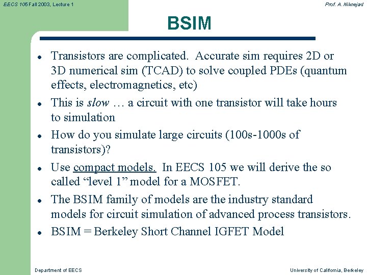
EECS 105 Fall 2003, Lecture 1 Prof. A. Niknejad BSIM l l l Transistors are complicated. Accurate sim requires 2 D or 3 D numerical sim (TCAD) to solve coupled PDEs (quantum effects, electromagnetics, etc) This is slow … a circuit with one transistor will take hours to simulation How do you simulate large circuits (100 s-1000 s of transistors)? Use compact models. In EECS 105 we will derive the so called “level 1” model for a MOSFET. The BSIM family of models are the industry standard models for circuit simulation of advanced process transistors. BSIM = Berkeley Short Channel IGFET Model Department of EECS University of California, Berkeley

EECS 105 Fall 2003, Lecture 1 Prof. A. Niknejad Berkeley… l A great place to study circuits, devices, and CAD! Department of EECS University of California, Berkeley

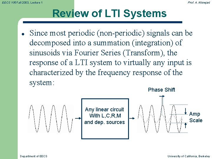
EECS 105 Fall 2003, Lecture 1 Prof. A. Niknejad Review of LTI Systems l Since most periodic (non-periodic) signals can be decomposed into a summation (integration) of sinusoids via Fourier Series (Transform), the response of a LTI system to virtually any input is characterized by the frequency response of the system: Phase Shift Any linear circuit With L, C, R, M and dep. sources Department of EECS Amp Scale University of California, Berkeley

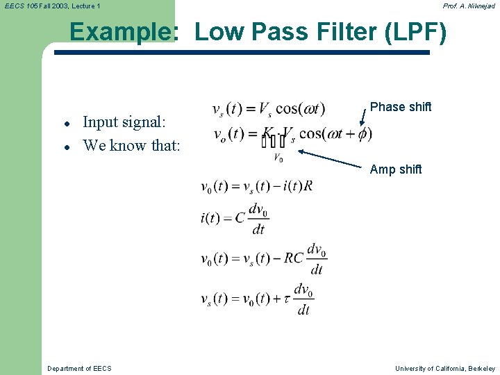
EECS 105 Fall 2003, Lecture 1 Prof. A. Niknejad Example: Low Pass Filter (LPF) l l Input signal: We know that: Phase shift Amp shift Department of EECS University of California, Berkeley

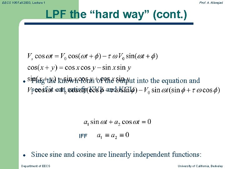
EECS 105 Fall 2003, Lecture 1 Prof. A. Niknejad LPF the “hard way” (cont. ) l Plug the known form of the output into the equation and see if it can satisfy KVL and KCL IFF l Since sine and cosine are linearly independent functions: Department of EECS University of California, Berkeley

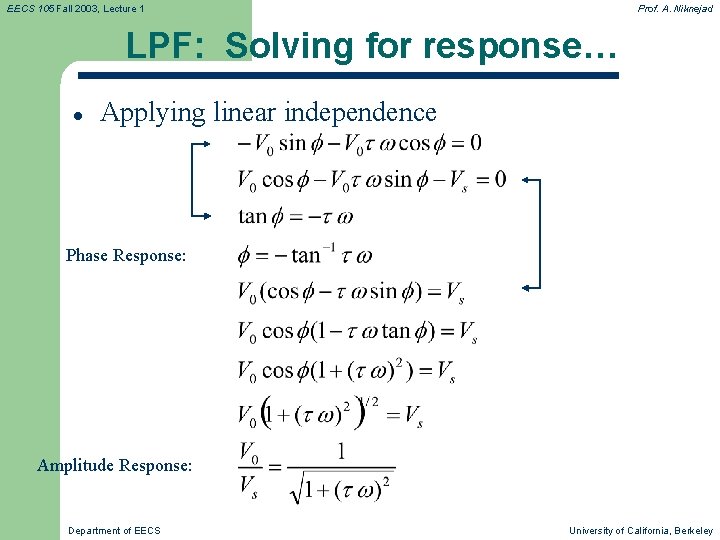
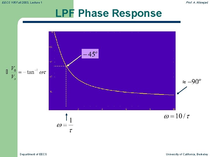
EECS 105 Fall 2003, Lecture 1 Prof. A. Niknejad LPF: Solving for response… l Applying linear independence Phase Response: Amplitude Response: Department of EECS University of California, Berkeley

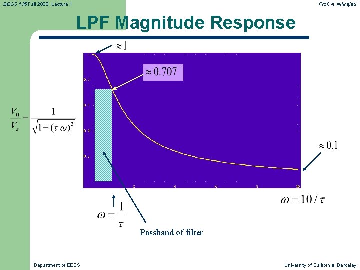
EECS 105 Fall 2003, Lecture 1 Prof. A. Niknejad LPF Magnitude Response Passband of filter Department of EECS University of California, Berkeley

EECS 105 Fall 2003, Lecture 1 Prof. A. Niknejad LPF Phase Response Department of EECS University of California, Berkeley

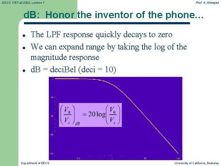
EECS 105 Fall 2003, Lecture 1 Prof. A. Niknejad d. B: Honor the inventor of the phone… l l l The LPF response quickly decays to zero We can expand range by taking the log of the magnitude response d. B = deci. Bel (deci = 10) Department of EECS University of California, Berkeley

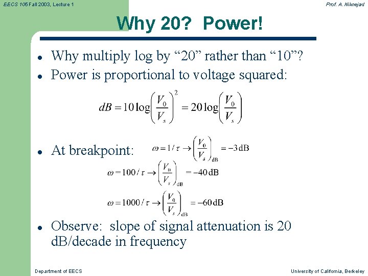
EECS 105 Fall 2003, Lecture 1 Prof. A. Niknejad Why 20? Power! l Why multiply log by “ 20” rather than “ 10”? Power is proportional to voltage squared: l At breakpoint: l l Observe: slope of signal attenuation is 20 d. B/decade in frequency Department of EECS University of California, Berkeley

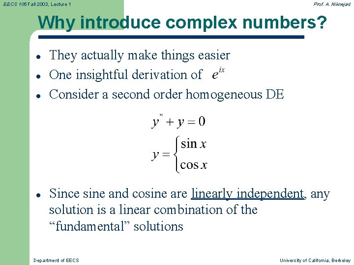
EECS 105 Fall 2003, Lecture 1 Prof. A. Niknejad Why introduce complex numbers? l l They actually make things easier One insightful derivation of Consider a second order homogeneous DE Since sine and cosine are linearly independent, any solution is a linear combination of the “fundamental” solutions Department of EECS University of California, Berkeley

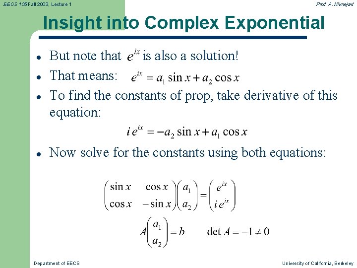
EECS 105 Fall 2003, Lecture 1 Prof. A. Niknejad Insight into Complex Exponential l l But note that is also a solution! That means: To find the constants of prop, take derivative of this equation: Now solve for the constants using both equations: Department of EECS University of California, Berkeley

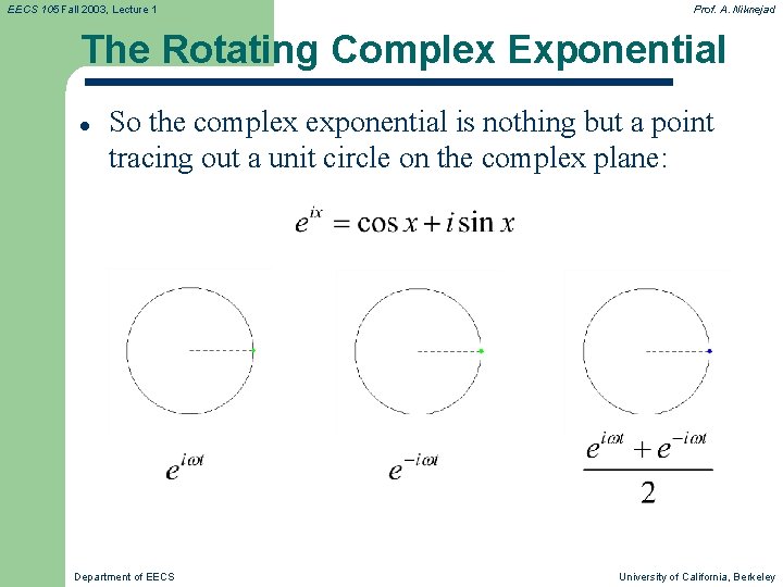
EECS 105 Fall 2003, Lecture 1 Prof. A. Niknejad The Rotating Complex Exponential l So the complex exponential is nothing but a point tracing out a unit circle on the complex plane: Department of EECS University of California, Berkeley

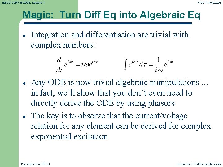
EECS 105 Fall 2003, Lecture 1 Prof. A. Niknejad Magic: Turn Diff Eq into Algebraic Eq l l l Integration and differentiation are trivial with complex numbers: Any ODE is now trivial algebraic manipulations … in fact, we’ll show that you don’t even need to directly derive the ODE by using phasors The key is to observe that the current/voltage relation for any element can be derived for complex exponential excitation Department of EECS University of California, Berkeley

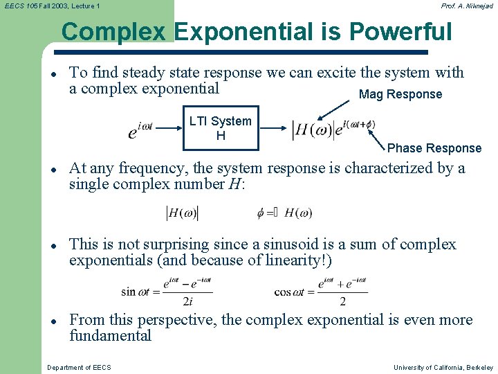
EECS 105 Fall 2003, Lecture 1 Prof. A. Niknejad Complex Exponential is Powerful l To find steady state response we can excite the system with a complex exponential Mag Response LTI System H l l l Phase Response At any frequency, the system response is characterized by a single complex number H: This is not surprising since a sinusoid is a sum of complex exponentials (and because of linearity!) From this perspective, the complex exponential is even more fundamental Department of EECS University of California, Berkeley

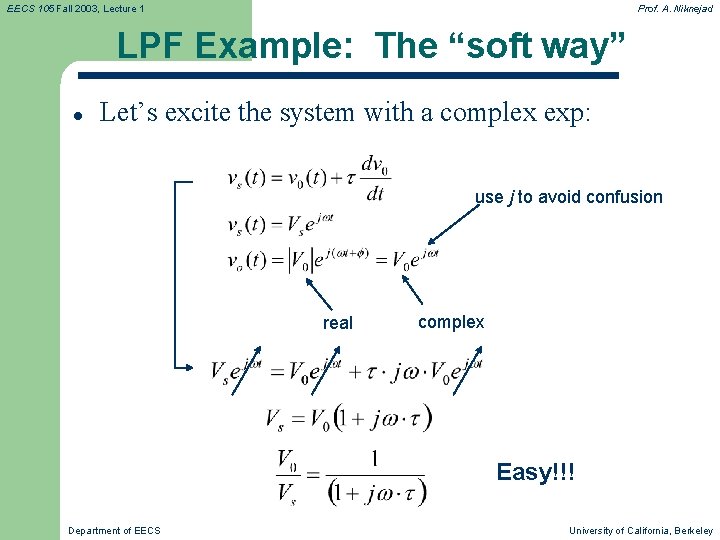
EECS 105 Fall 2003, Lecture 1 Prof. A. Niknejad LPF Example: The “soft way” l Let’s excite the system with a complex exp: use j to avoid confusion real complex Easy!!! Department of EECS University of California, Berkeley

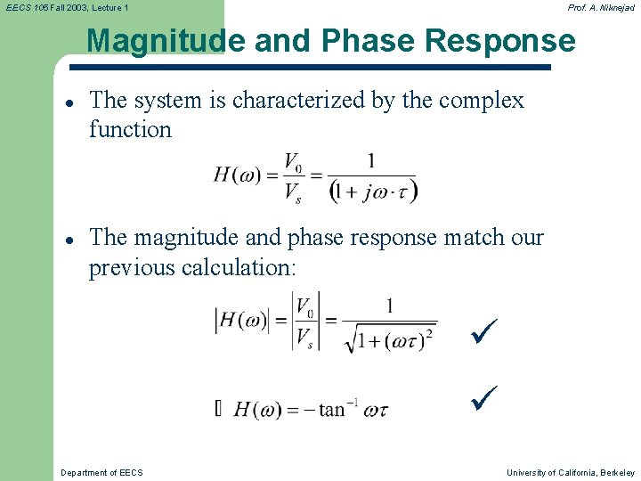
EECS 105 Fall 2003, Lecture 1 Prof. A. Niknejad Magnitude and Phase Response l l The system is characterized by the complex function The magnitude and phase response match our previous calculation: Department of EECS University of California, Berkeley

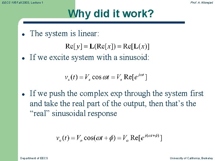
EECS 105 Fall 2003, Lecture 1 Prof. A. Niknejad Why did it work? l The system is linear: l If we excite system with a sinusoid: l If we push the complex exp through the system first and take the real part of the output, then that’s the “real” sinusoidal response Department of EECS University of California, Berkeley

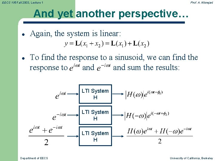
EECS 105 Fall 2003, Lecture 1 Prof. A. Niknejad And yet another perspective… l l Again, the system is linear: To find the response to a sinusoid, we can find the response to and sum the results: LTI System H Department of EECS University of California, Berkeley

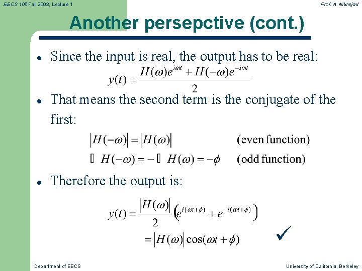
EECS 105 Fall 2003, Lecture 1 Prof. A. Niknejad Another persepctive (cont. ) l l l Since the input is real, the output has to be real: That means the second term is the conjugate of the first: Therefore the output is: Department of EECS University of California, Berkeley

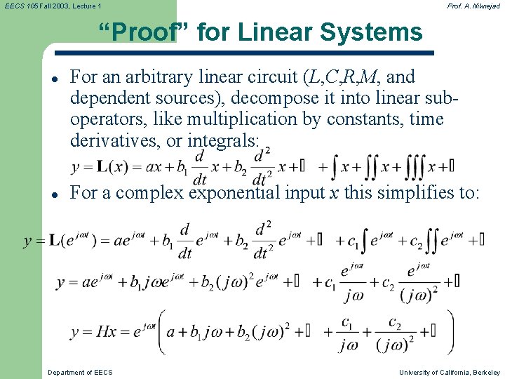
EECS 105 Fall 2003, Lecture 1 Prof. A. Niknejad “Proof” for Linear Systems l l For an arbitrary linear circuit (L, C, R, M, and dependent sources), decompose it into linear suboperators, like multiplication by constants, time derivatives, or integrals: For a complex exponential input x this simplifies to: Department of EECS University of California, Berkeley

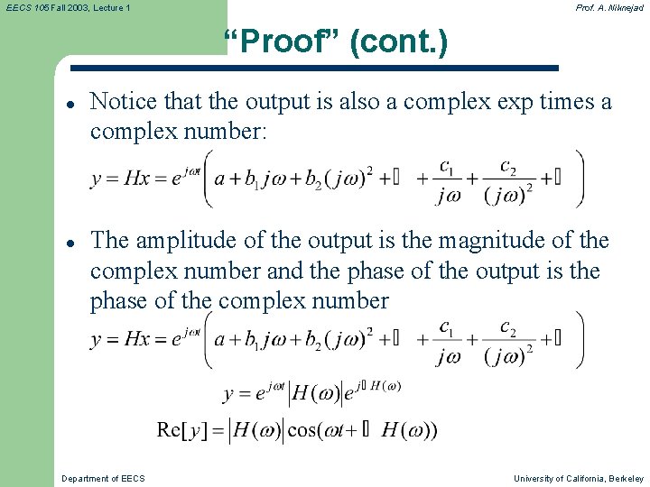
EECS 105 Fall 2003, Lecture 1 Prof. A. Niknejad “Proof” (cont. ) l l Notice that the output is also a complex exp times a complex number: The amplitude of the output is the magnitude of the complex number and the phase of the output is the phase of the complex number Department of EECS University of California, Berkeley

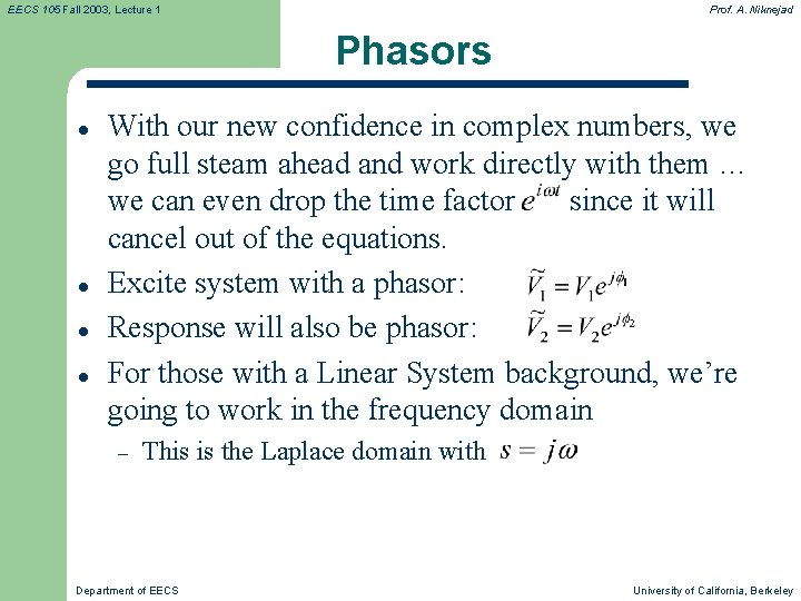
EECS 105 Fall 2003, Lecture 1 Prof. A. Niknejad Phasors l l With our new confidence in complex numbers, we go full steam ahead and work directly with them … we can even drop the time factor since it will cancel out of the equations. Excite system with a phasor: Response will also be phasor: For those with a Linear System background, we’re going to work in the frequency domain – This is the Laplace domain with Department of EECS University of California, Berkeley

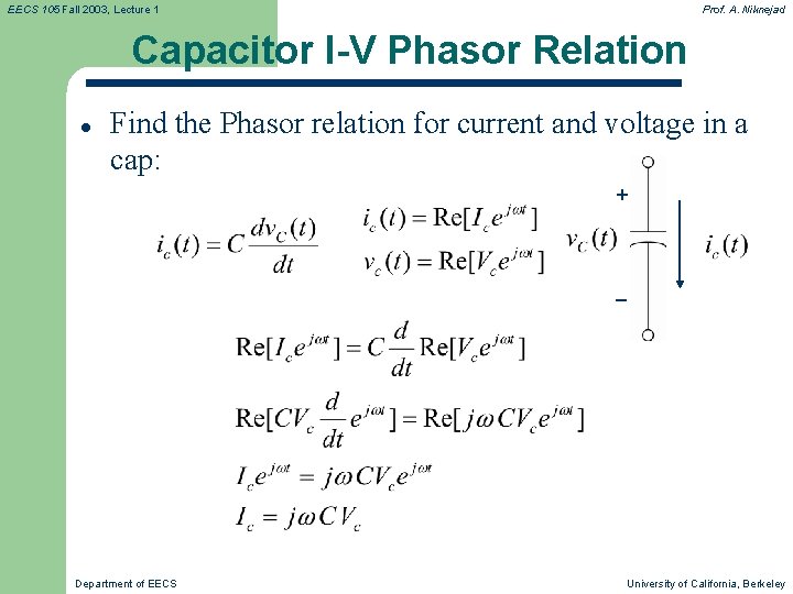
EECS 105 Fall 2003, Lecture 1 Prof. A. Niknejad Capacitor I-V Phasor Relation l Find the Phasor relation for current and voltage in a cap: + _ Department of EECS University of California, Berkeley

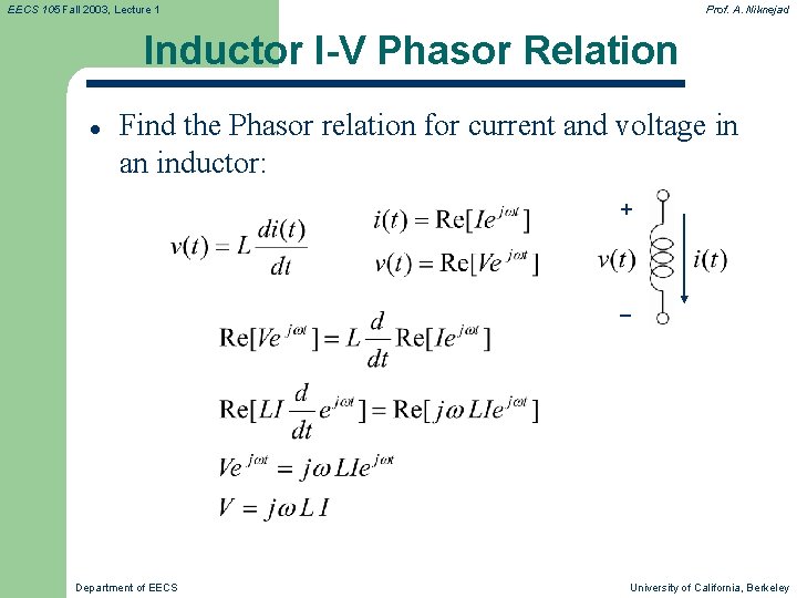
EECS 105 Fall 2003, Lecture 1 Prof. A. Niknejad Inductor I-V Phasor Relation l Find the Phasor relation for current and voltage in an inductor: + _ Department of EECS University of California, Berkeley