EE565 Mobile Robotics NonParametric Filters Module 2 Lecture

EE-565: Mobile Robotics Non-Parametric Filters Module 2, Lecture 5 Dr Abubakr Muhammad Assistant Professor Electrical Engineering, LUMS Director, CYPHYNETS Lab http: //cyphynets. lums. edu. pk SA-1 9 -1

Resources Course material from • Stanford CS-226 (Thrun) [slides] • KAUST ME-410 (Abubakr, 2011) • LUMS EE-662 (Abubakr, 2013) http: //cyphynets. lums. edu. pk/index. php/Teaching Textbooks • Probabilistic Robotics by Thrun et al. • Principles of Robot Motion by Choset et al. 9 -2

Part 1. BAYESIAN PHILOSOPHY FOR STATE ESTIMATION 9 -3

State Estimation Problems • What is a state? • Inferring “hidden states” from observations • What if observations are noisy? • More challenging, if state is also dynamic. • Even more challenging, if the state dynamics are also noisy. 9 -4

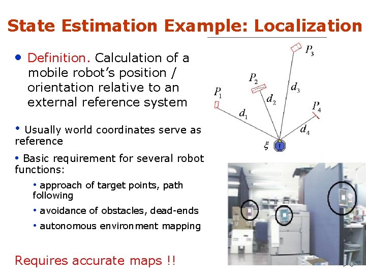
State Estimation Example: Localization • Definition. Calculation of a mobile robot’s position / orientation relative to an external reference system • Usually world coordinates serve as reference • Basic requirement for several robot functions: • approach of target points, path following • avoidance of obstacles, dead-ends • autonomous environment mapping Requires accurate maps !! 9 -5

State Estimation Example: Mapping • Objective: Store information • outside of sensory horizon Map provided a-priori or can be online • Types • world-centric maps navigation, path planning • robot-centric maps pilot tasks (e. g. collision avoidance) • Problem: inaccuracy due to sensor systems Requires accurate localization!! 9 -6

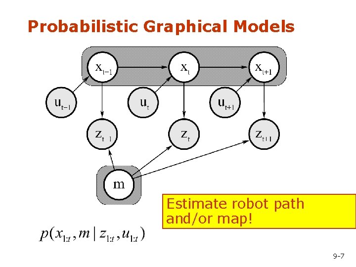
Probabilistic Graphical Models Estimate robot path and/or map! 9 -7

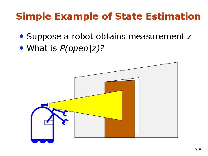
Simple Example of State Estimation • Suppose a robot obtains measurement z • What is P(open|z)? 9 -8

Bayes Formula 9 -9

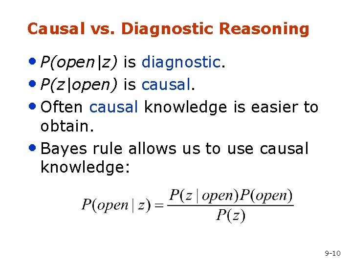
Causal vs. Diagnostic Reasoning • P(open|z) is diagnostic. • P(z|open) is causal. • Often causal knowledge is easier to obtain. • Bayes rule allows us to use causal knowledge: 9 -10

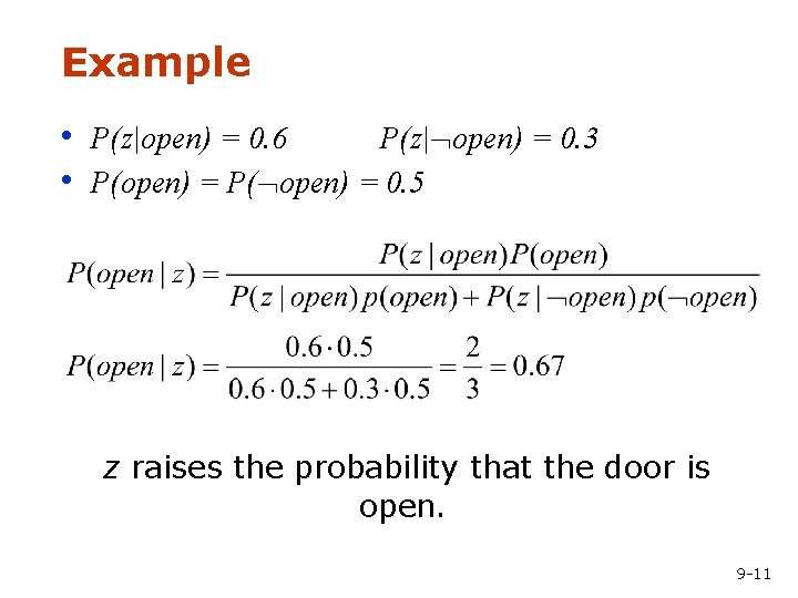
Example • P(z|open) = 0. 6 P(z| open) = 0. 3 • P(open) = P( open) = 0. 5 z raises the probability that the door is open. 9 -11

Combining Evidence • Suppose our robot obtains another observation z 2. • How can we integrate this new information? • More generally, how can we estimate P(x| z 1. . . zn )? 9 -12

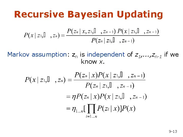
Recursive Bayesian Updating Markov assumption: zn is independent of z 1, . . . , zn-1 if we know x. 9 -13

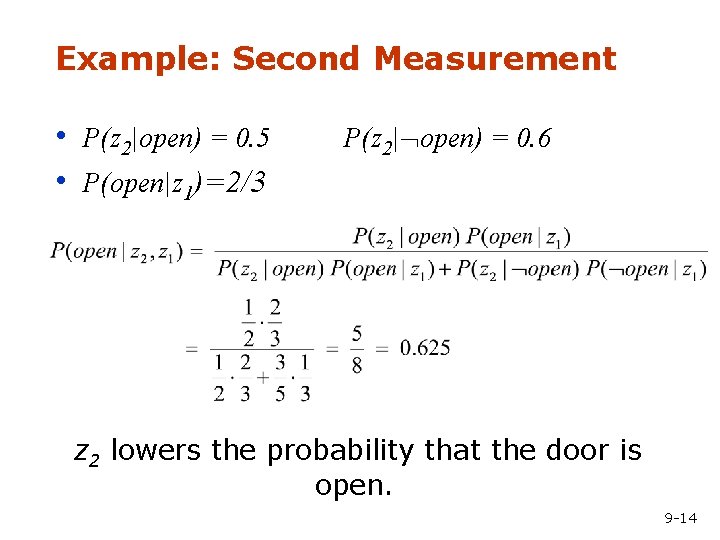
Example: Second Measurement • P(z 2|open) = 0. 5 • P(open|z 1)=2/3 P(z 2| open) = 0. 6 z 2 lowers the probability that the door is open. 9 -14

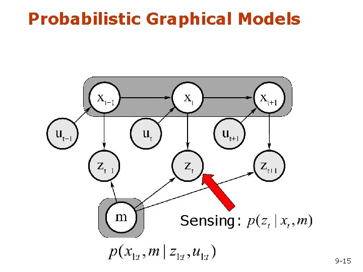
Probabilistic Graphical Models Sensing: 9 -15

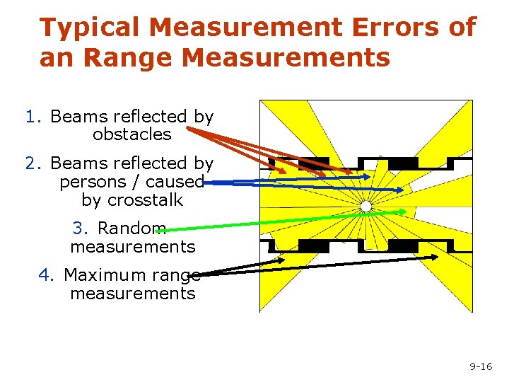
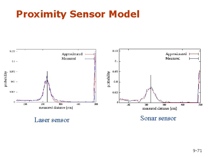
Typical Measurement Errors of an Range Measurements 1. Beams reflected by obstacles 2. Beams reflected by persons / caused by crosstalk 3. Random measurements 4. Maximum range measurements 9 -16

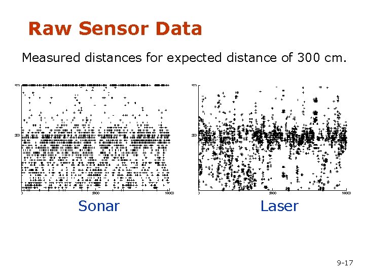
Raw Sensor Data Measured distances for expected distance of 300 cm. Sonar Laser 9 -17

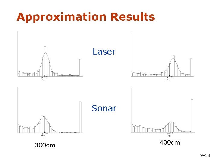
Approximation Results Laser Sonar 300 cm 400 cm 9 -18

Actions • Often the world is dynamic since • actions carried out by the robot, • actions carried out by other agents, • or just the time passing by change the world. • How can we incorporate such actions? 9 -19

Typical Actions • The robot turns its wheels to move • The robot uses its manipulator to grasp • an object Plants grow over time… • Actions are never carried out with • absolute certainty. In contrast to measurements, actions generally increase the uncertainty. 9 -20

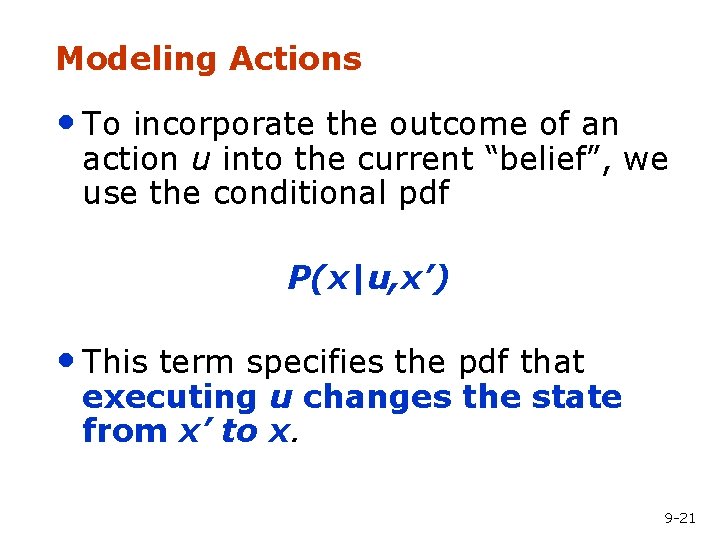
Modeling Actions • To incorporate the outcome of an action u into the current “belief”, we use the conditional pdf P(x|u, x’) • This term specifies the pdf that executing u changes the state from x’ to x. 9 -21

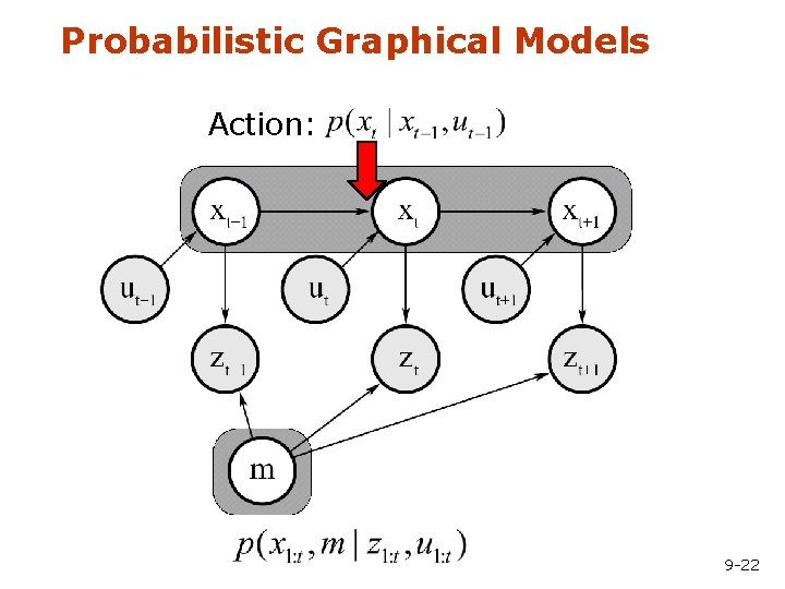
Probabilistic Graphical Models Action: 9 -22

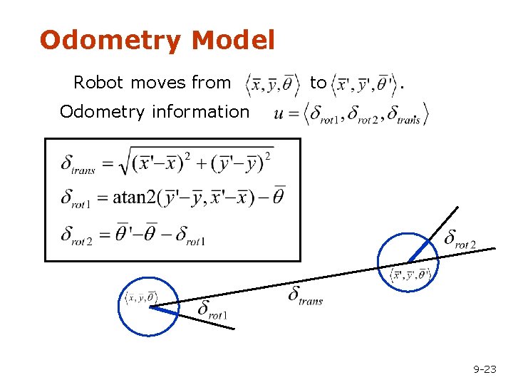
Odometry Model Robot moves from Odometry information to . . 9 -23

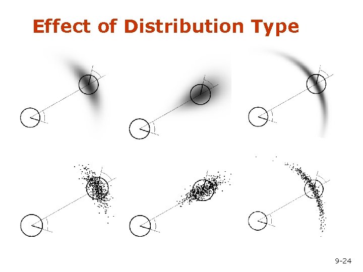
Effect of Distribution Type 9 -24

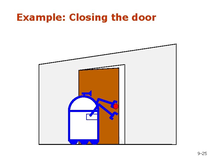
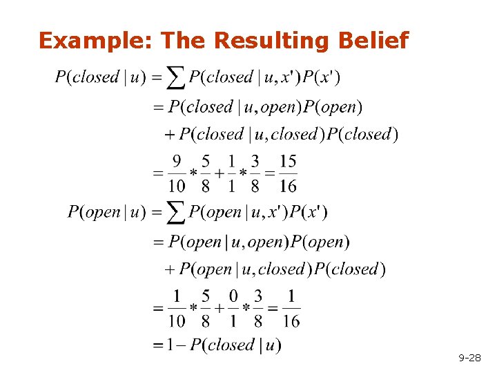
Example: Closing the door 9 -25

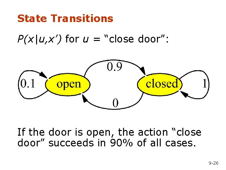
State Transitions P(x|u, x’) for u = “close door”: If the door is open, the action “close door” succeeds in 90% of all cases. 9 -26

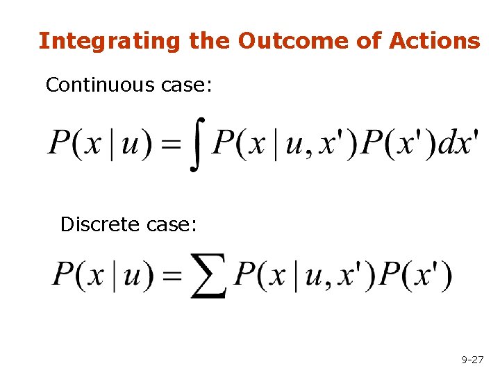
Integrating the Outcome of Actions Continuous case: Discrete case: 9 -27

Example: The Resulting Belief 9 -28

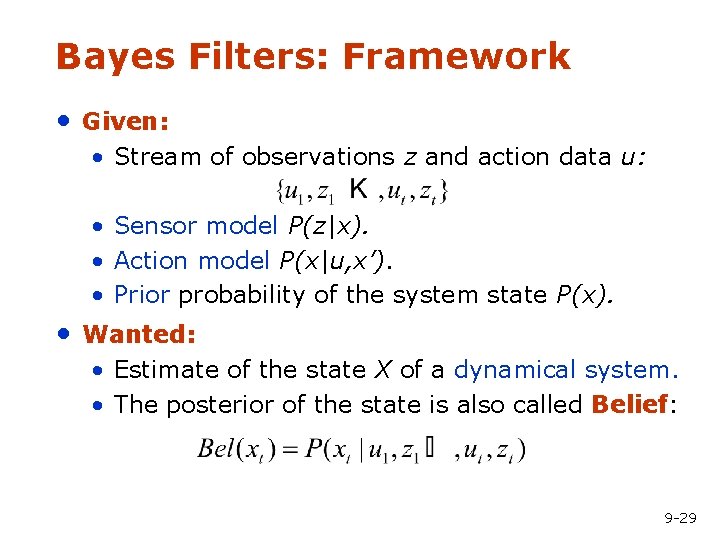
Bayes Filters: Framework • Given: • Stream of observations z and action data u: • Sensor model P(z|x). • Action model P(x|u, x’). • Prior probability of the system state P(x). • Wanted: • Estimate of the state X of a dynamical system. • The posterior of the state is also called Belief: 9 -29

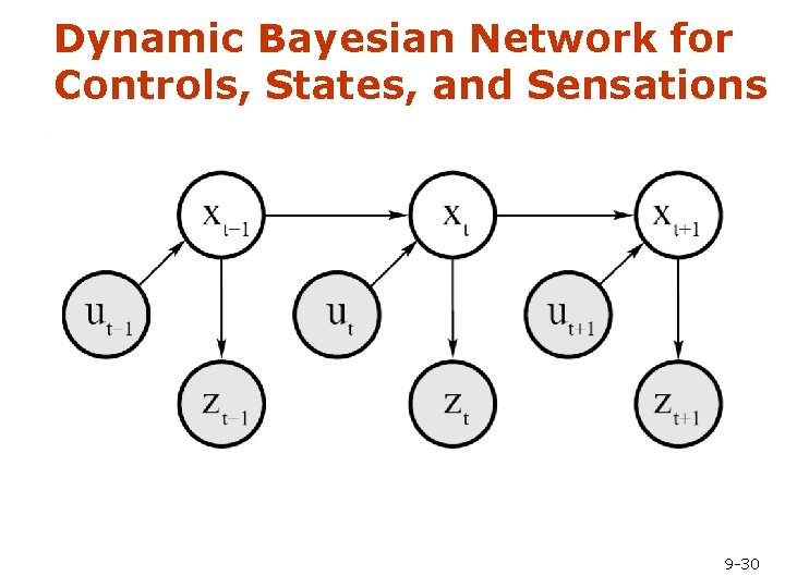
Dynamic Bayesian Network for Controls, States, and Sensations 9 -30

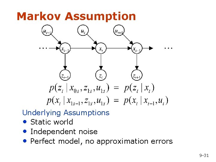
Markov Assumption Underlying Assumptions • Static world • Independent noise • Perfect model, no approximation errors 9 -31

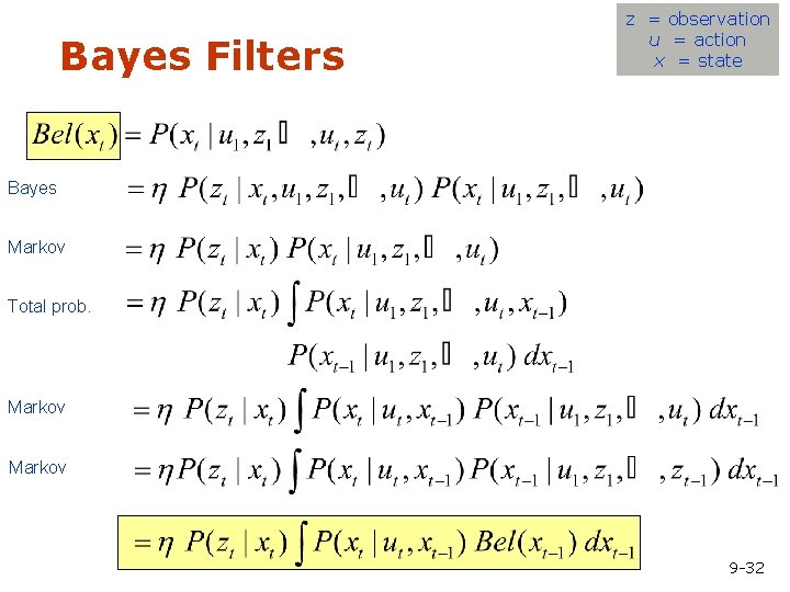
Bayes Filters z = observation u = action x = state Bayes Markov Total prob. Markov 9 -32

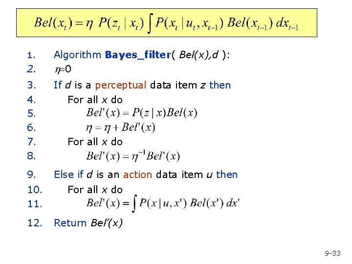
Bayes Filter Algorithm 1. 2. Algorithm Bayes_filter( Bel(x), d ): h=0 3. 4. 5. 6. 7. 8. If d is a perceptual data item z then For all x do 9. Else if d is an action data item u then For all x do 10. 11. For all x do 12. Return Bel’(x) 9 -33

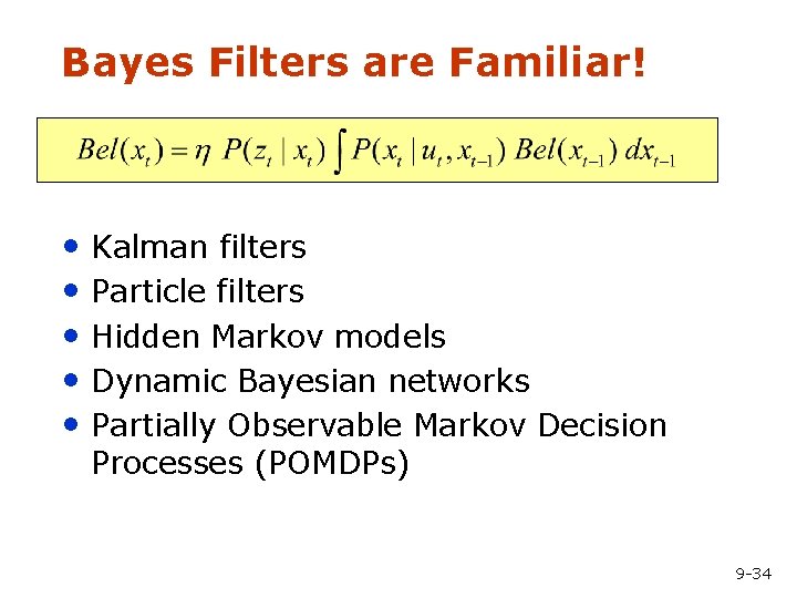
Bayes Filters are Familiar! • Kalman filters • Particle filters • Hidden Markov models • Dynamic Bayesian networks • Partially Observable Markov Decision Processes (POMDPs) 9 -34

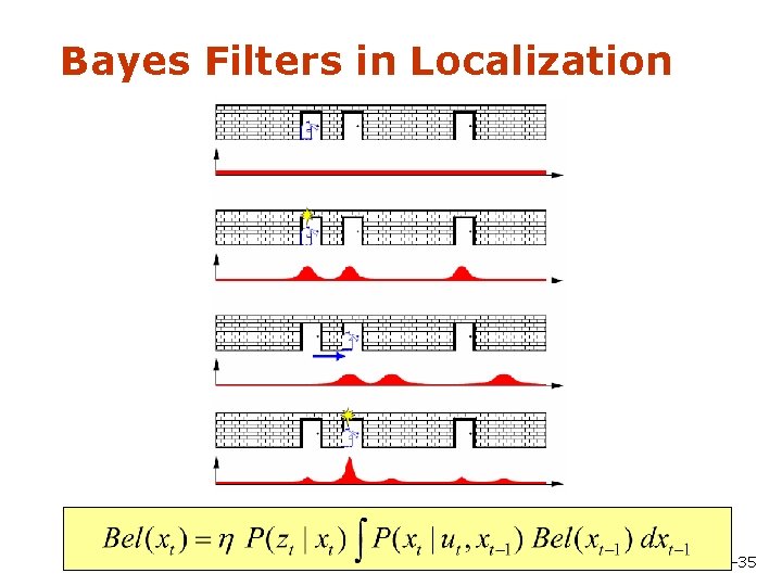
Bayes Filters in Localization 9 -35

Summary so far …. • Bayes rule allows us to compute probabilities that are hard to assess otherwise. • Under the Markov assumption, recursive Bayesian updating can be used to efficiently combine evidence. • Bayes filters are a probabilistic tool for estimating the state of dynamic systems. 9 -36

Parametric Vs. Non-parametric • Representing distributions by using statistics or parameters (mean, variance) • Non-parametric approach: Deal with distributions directly • Remember: 1. Gaussian distribution is completely parameterized by two numbers (mean, variance) 2. Gaussian distribution remains Gaussian when mapped linearly. 9 -37

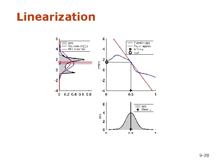
Linearization 9 -38

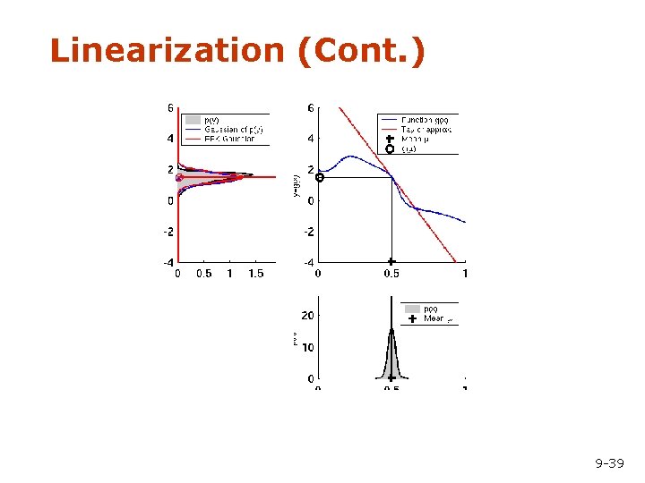
Linearization (Cont. ) 9 -39

Bayes Filters in Localization 9 -40

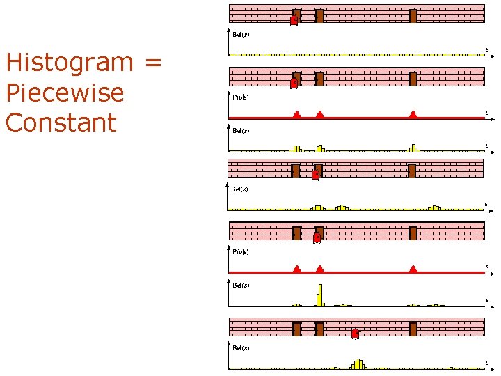
Histogram = Piecewise Constant 41 9 -41

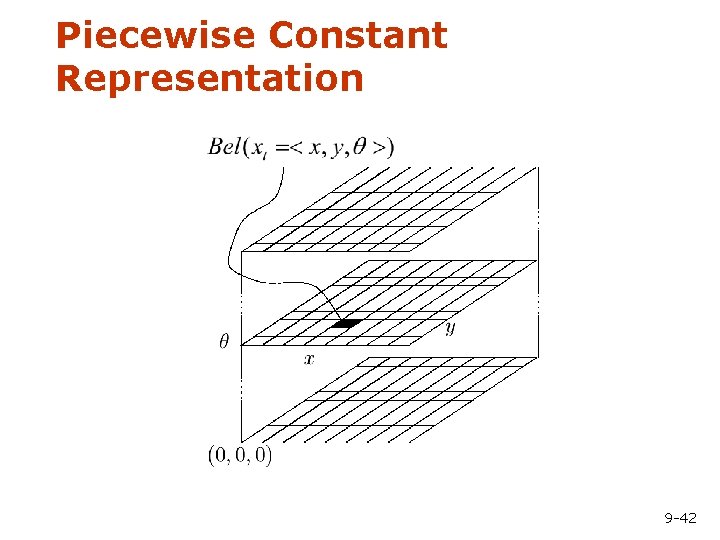
Piecewise Constant Representation 9 -42

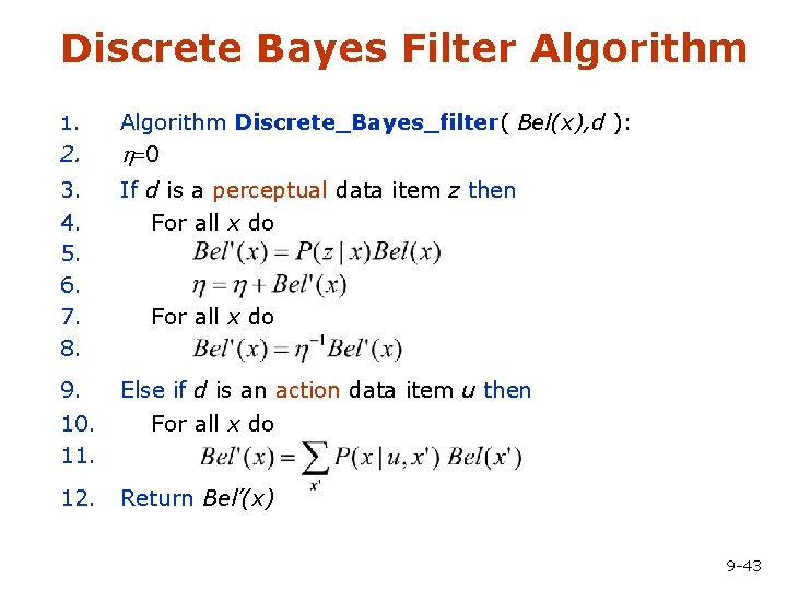
Discrete Bayes Filter Algorithm 1. 2. Algorithm Discrete_Bayes_filter( Bel(x), d ): h=0 3. 4. 5. 6. 7. 8. If d is a perceptual data item z then For all x do 9. Else if d is an action data item u then For all x do 10. 11. For all x do 12. Return Bel’(x) 9 -43

Implementation (1) • To update the belief upon sensory input and to carry out the normalization one has to iterate over all cells of the grid. • Especially when the belief is peaked (which is generally the case during position tracking), one wants to avoid updating irrelevant aspects of the state space. • One approach is not to update entire sub-spaces of the state space. • This, however, requires to monitor whether the robot is de -localized or not. • To achieve this, one can consider the likelihood of the observations given the active components of the state space. 9 -44

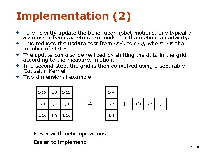
Implementation (2) • To efficiently update the belief upon robot motions, one typically • • assumes a bounded Gaussian model for the motion uncertainty. This reduces the update cost from O(n 2) to O(n), where n is the number of states. The update can also be realized by shifting the data in the grid according to the measured motion. In a second step, the grid is then convolved using a separable Gaussian Kernel. Two-dimensional example: 1/16 1/8 1/4 1/8 1/16 1/4 1/2 + 1/4 1/2 1/4 Fewer arithmetic operations Easier to implement 9 -45

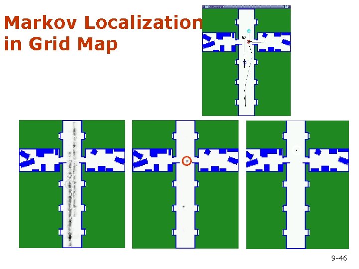
Markov Localization in Grid Map 9 -46

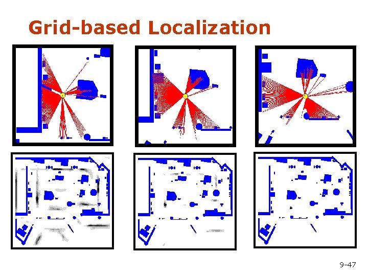
Grid-based Localization 9 -47

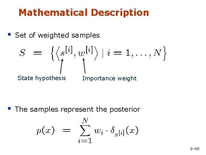
Mathematical Description § Set of weighted samples State hypothesis § Importance weight The samples represent the posterior 9 -48

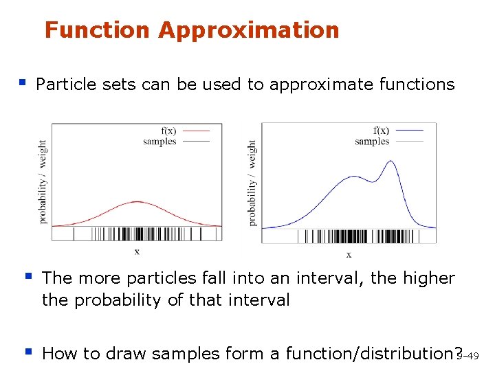
Function Approximation § Particle sets can be used to approximate functions § The more particles fall into an interval, the higher the probability of that interval § How to draw samples form a function/distribution? 9 -49

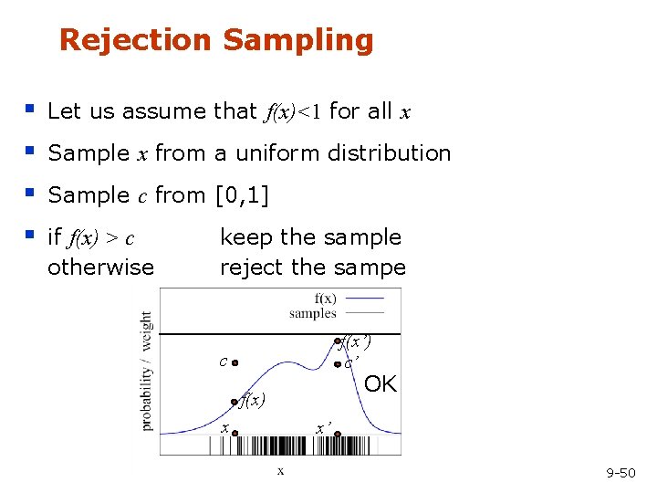
Rejection Sampling § § Let us assume that f(x)<1 for all x Sample x from a uniform distribution Sample c from [0, 1] if f(x) > c otherwise keep the sample reject the sampe f(x’) c’ c OK f(x) x x’ 9 -50

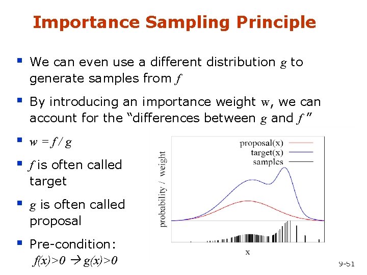
Importance Sampling Principle § We can even use a different distribution g to generate samples from f § By introducing an importance weight w, we can account for the “differences between g and f ” § § w=f/g § g is often called proposal § Pre-condition: f(x)>0 g(x)>0 f is often called target 9 -51

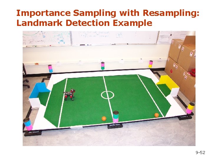
Importance Sampling with Resampling: Landmark Detection Example 9 -52

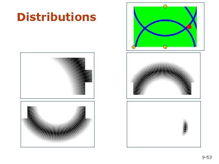
Distributions 9 -53

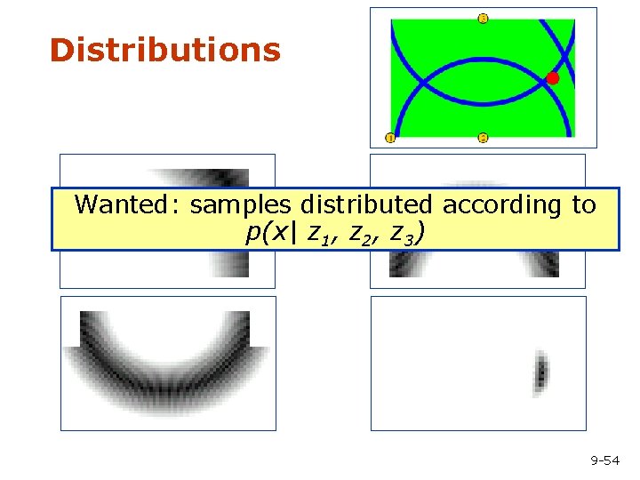
Distributions Wanted: samples distributed according to p(x| z 1, z 2, z 3) 9 -54

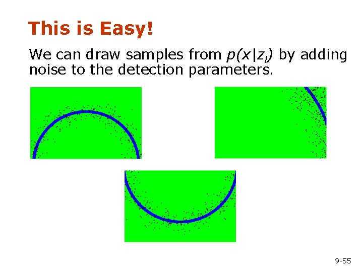
This is Easy! We can draw samples from p(x|zl) by adding noise to the detection parameters. 9 -55

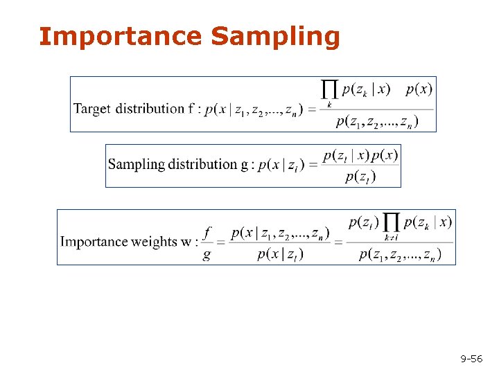
Importance Sampling 9 -56

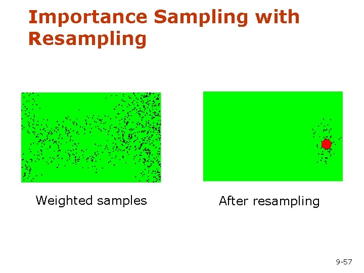
Importance Sampling with Resampling Weighted samples After resampling 9 -57

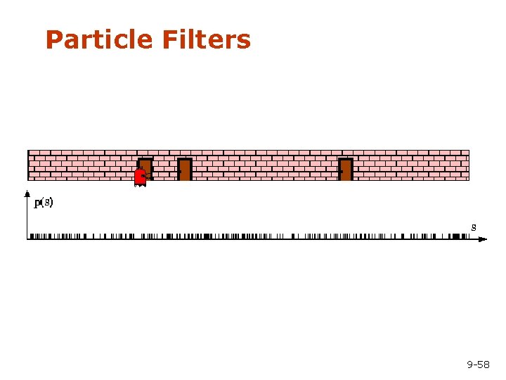
Particle Filters 9 -58

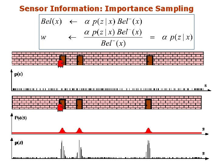
Sensor Information: Importance Sampling 9 -59

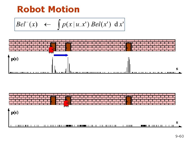
Robot Motion 9 -60

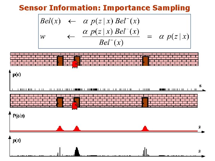
Sensor Information: Importance Sampling 9 -61

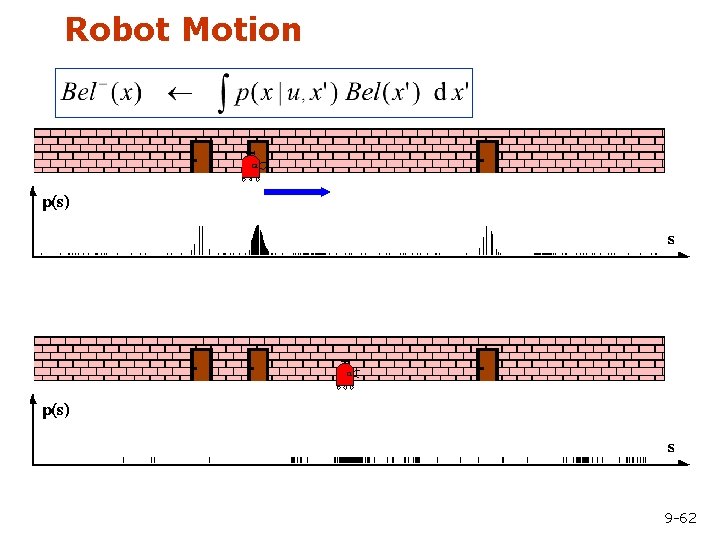
Robot Motion 9 -62

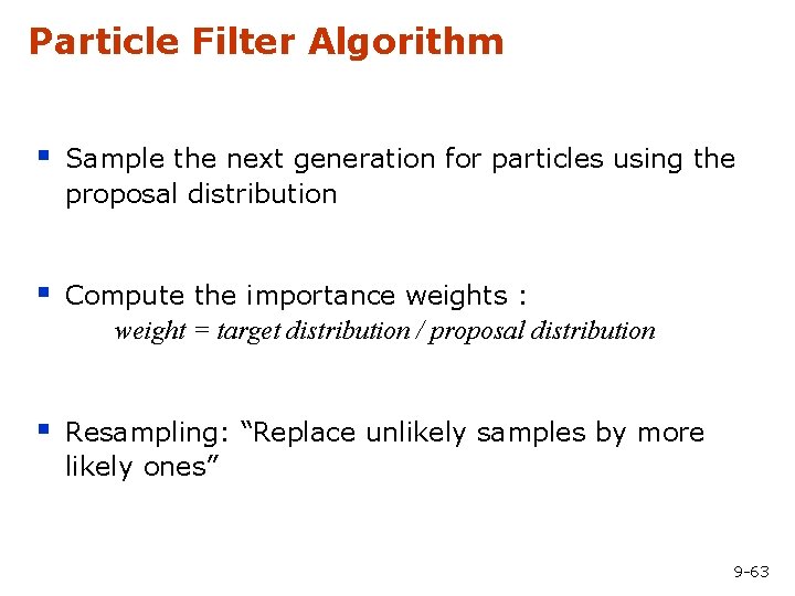
Particle Filter Algorithm § Sample the next generation for particles using the proposal distribution § Compute the importance weights : weight = target distribution / proposal distribution § Resampling: “Replace unlikely samples by more likely ones” 9 -63

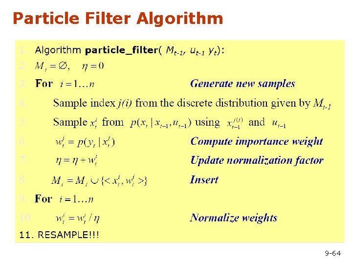
Particle Filter Algorithm 9 -64

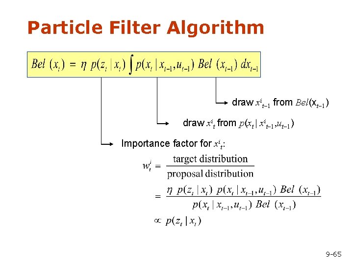
Particle Filter Algorithm draw xit-1 from Bel(xt-1) draw xit from p(xt | xit-1, ut-1) Importance factor for xit: 9 -65

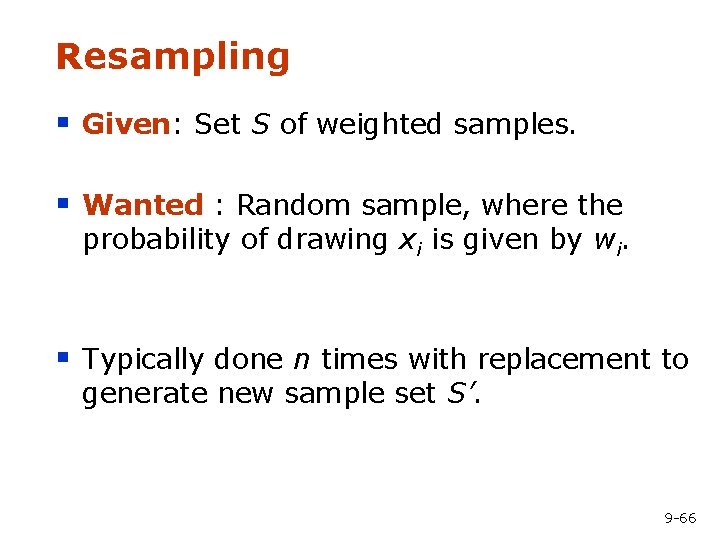
Resampling § Given: Set S of weighted samples. § Wanted : Random sample, where the probability of drawing xi is given by wi. § Typically done n times with replacement to generate new sample set S’. 9 -66

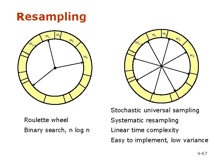
Resampling wn wn w 1 Wn-1 w 2 w 3 Stochastic universal sampling Roulette wheel Systematic resampling Binary search, n log n Linear time complexity Easy to implement, low variance 9 -67

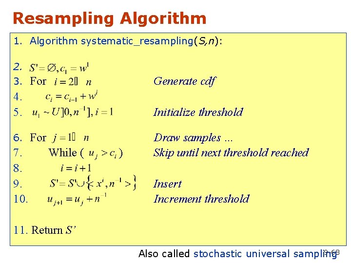
Resampling Algorithm 1. Algorithm systematic_resampling(S, n): 2. 3. For Generate cdf 4. 5. Initialize threshold 6. For 7. 8. 9. 10. While ( ) Draw samples … Skip until next threshold reached Insert Increment threshold 11. Return S’ 9 -68 Also called stochastic universal sampling

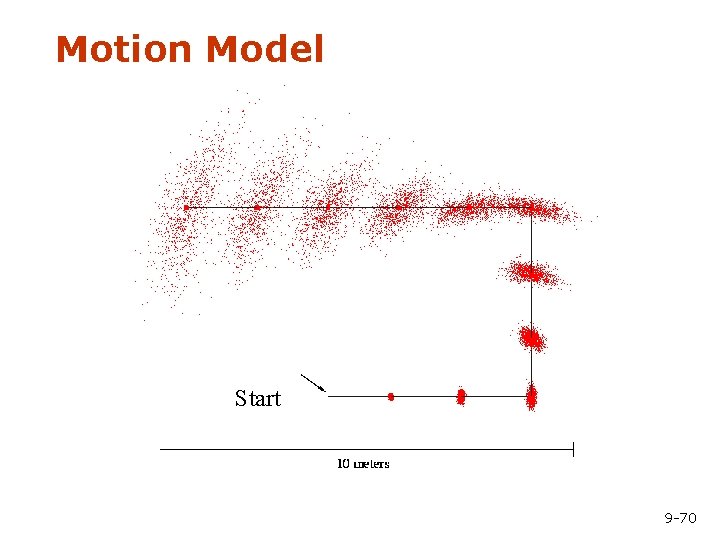
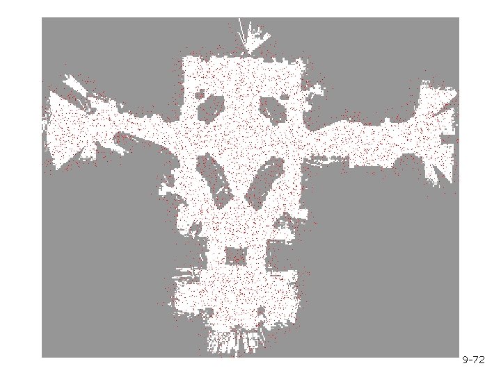
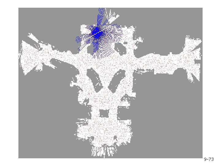
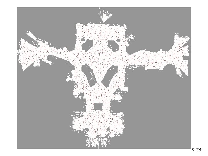
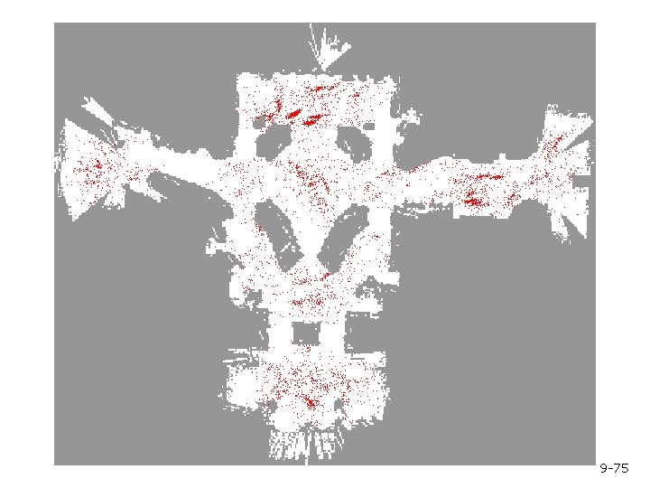
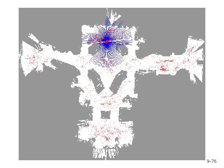
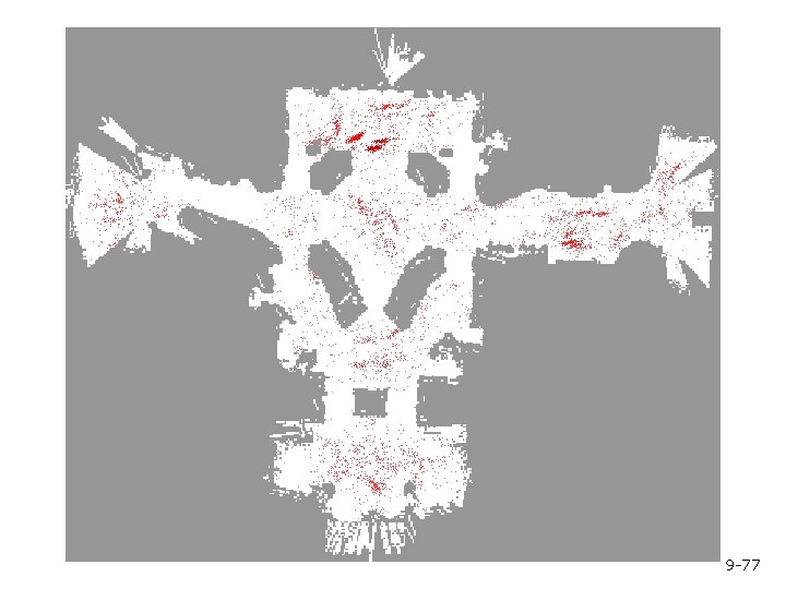
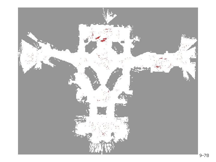
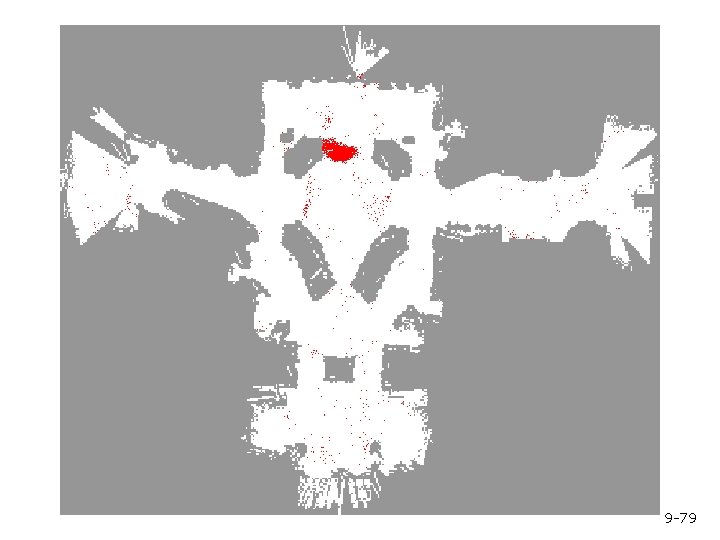
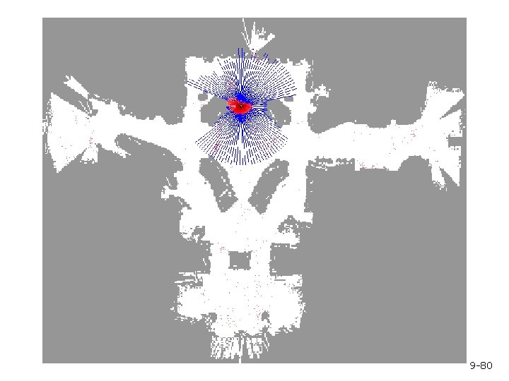
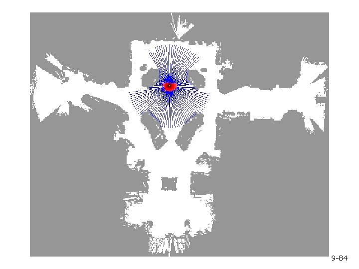
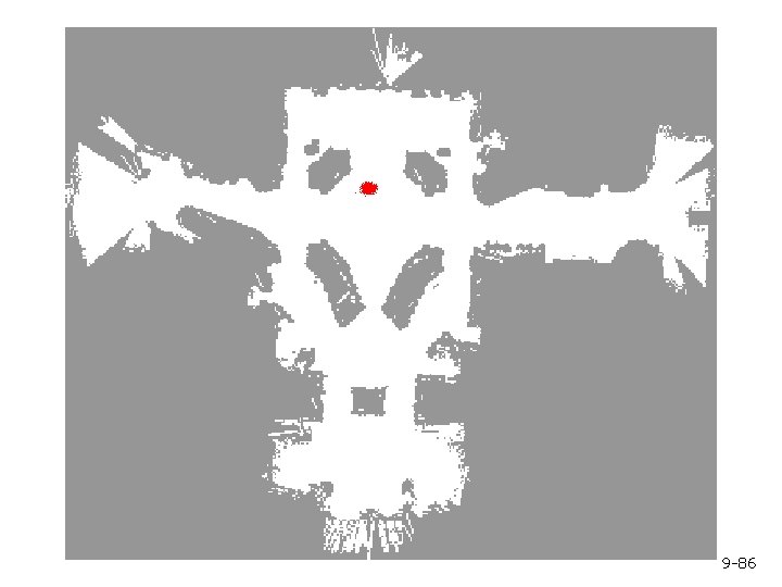
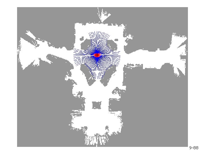
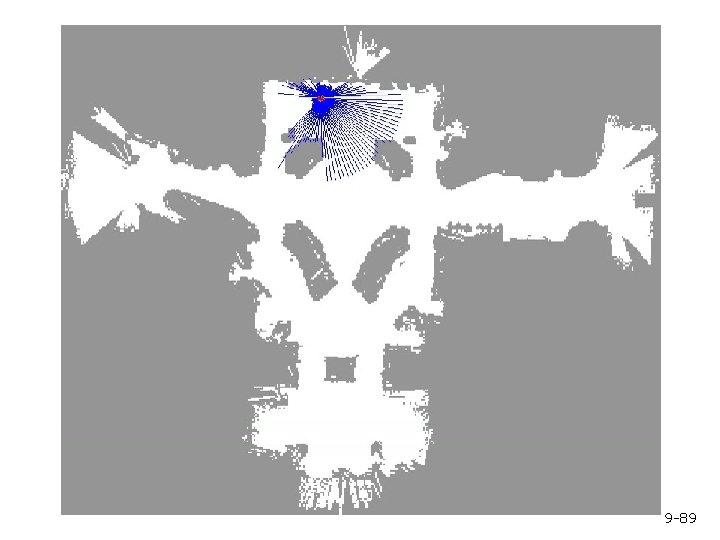
Mobile Robot Localization § Each particle is a potential pose of the robot § Proposal distribution is the motion model of the robot (prediction step) § The observation model is used to compute the importance weight (correction step) 9 -69

Motion Model Start 9 -70

Proximity Sensor Model Laser sensor Sonar sensor 9 -71

9 -72

9 -73

9 -74

9 -75

9 -76

9 -77

9 -78

9 -79

9 -80

9 -81

9 -82

9 -83

9 -84

9 -85

9 -86

9 -87

9 -88

9 -89

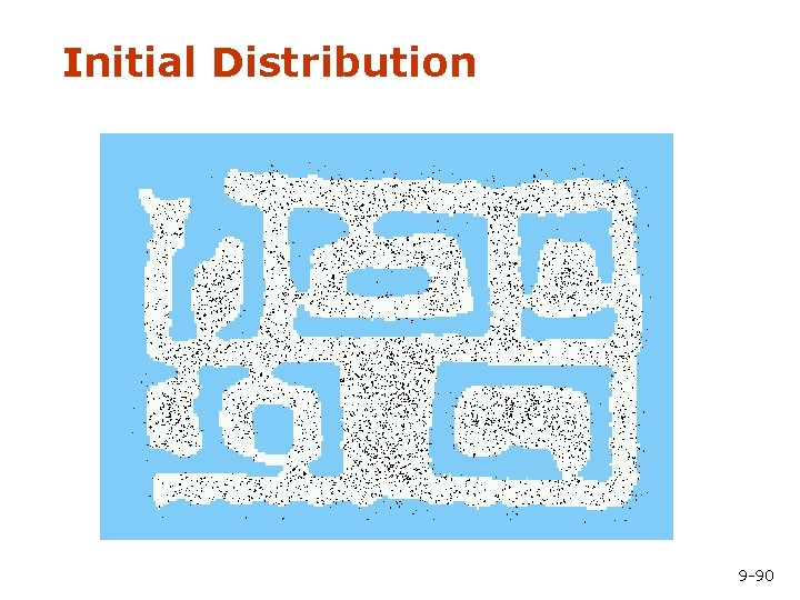
Initial Distribution 9 -90

After Incorporating Ten Ultrasound Scans 9 -91

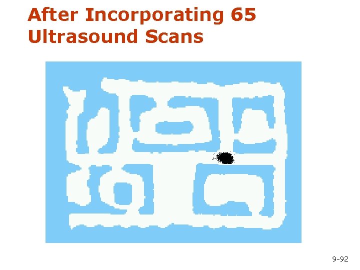
After Incorporating 65 Ultrasound Scans 9 -92

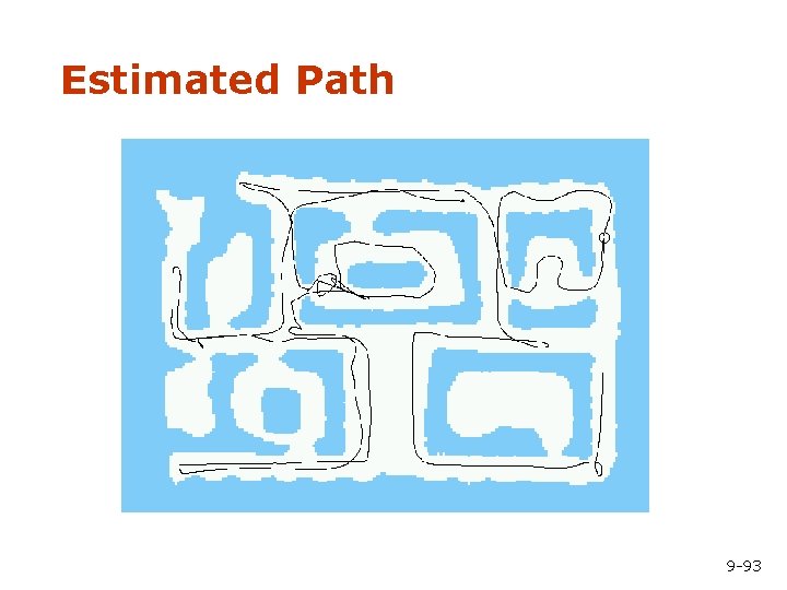
Estimated Path 9 -93

Using Ceiling Maps for Localization 9 -94 [Dellaert et al. 99]

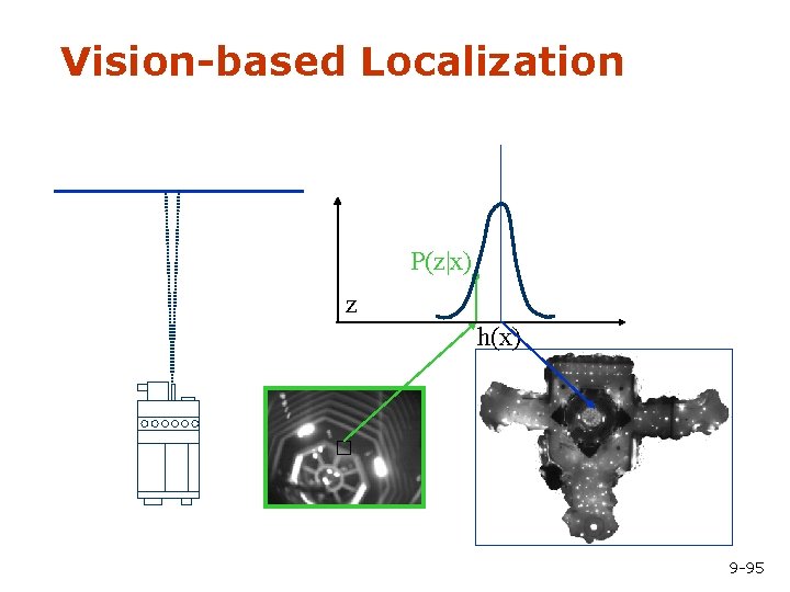
Vision-based Localization P(z|x) z h(x) 9 -95

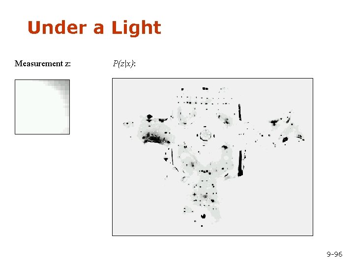
Under a Light Measurement z: P(z|x): 9 -96

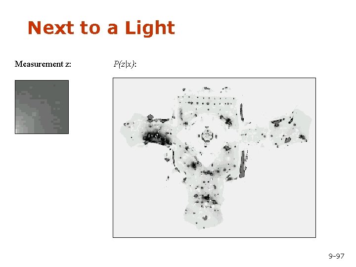
Next to a Light Measurement z: P(z|x): 9 -97

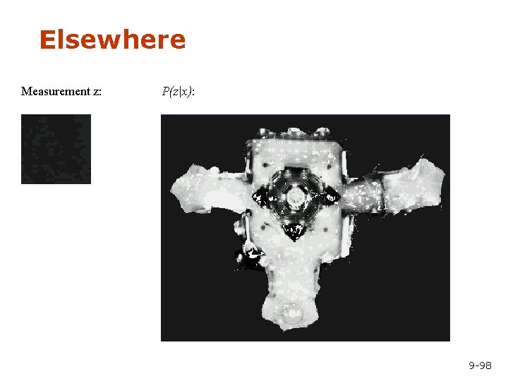
Elsewhere Measurement z: P(z|x): 9 -98

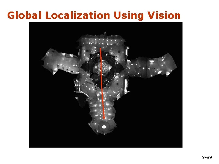
Global Localization Using Vision 9 -99

Summary – Particle Filters § Particle filters are an implementation of § § § recursive Bayesian filtering They represent the posterior by a set of weighted samples They can model non-Gaussian distributions Proposal to draw new samples Weight to account for the differences between the proposal and the target Monte Carlo filter, Survival of the fittest, Condensation, Bootstrap filter 9 -100

Summary – Monte Carlo Localization § In the context of localization, the § § particles are propagated according to the motion model. They are then weighted according to the likelihood of the observations. In a re-sampling step, new particles are drawn with a probability proportional to the likelihood of the observation. 9 -101