EE 368 Soft Computing Genetic Algorithms Outline Genetic

EE 368 Soft Computing Genetic Algorithms

Outline • Genetic Algorithms • Basic Components • General Structure • Example • Economic Load Dispatch problem using GA • MATLAB code for ELD using GA 2

Genetic Algorithms • Genetic algorithms are a particular class of evolutionary algorithms that use techniques inspired by evolutionary biology such as inheritance, mutation, selection, and crossover (also called recombination). • Genetic algorithms are implemented as a computer simulation in which a population of abstract representations (called chromosomes) of candidate solutions (called individuals) to an optimization problem evolves toward better solutions. • Traditionally, solutions are represented in binary as strings of 0 s and 1 s, but other encodings are also possible. 3

Genetic Algorithms • The evolution usually starts from a population of randomly generated individuals and happens in generations. • In each generation, the fitness of every individual in the population is evaluated, multiple individuals are selected from the current population (based on their fitness), and modified (recombined and possibly mutated) to form a new population. • The new population is then used in the next iteration of the algorithm. • Commonly, the algorithm terminates when either a maximum number of generations has been produced, or a satisfactory fitness level has been reached for the population. 4

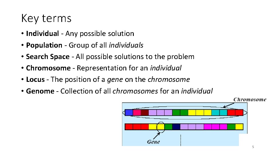
Key terms • Individual - Any possible solution • Population - Group of all individuals • Search Space - All possible solutions to the problem • Chromosome - Representation for an individual • Locus - The position of a gene on the chromosome • Genome - Collection of all chromosomes for an individual 5

GA Requirements • A typical genetic algorithm requires two things to be defined: • a genetic representation of the solution domain, and • a fitness function to evaluate the solution domain. 6

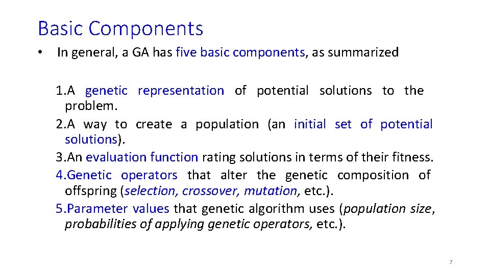
Basic Components • In general, a GA has five basic components, as summarized 1. A genetic representation of potential solutions to the problem. 2. A way to create a population (an initial set of potential solutions). 3. An evaluation function rating solutions in terms of their fitness. 4. Genetic operators that alter the genetic composition of offspring (selection, crossover, mutation, etc. ). 5. Parameter values that genetic algorithm uses (population size, probabilities of applying genetic operators, etc. ). 7

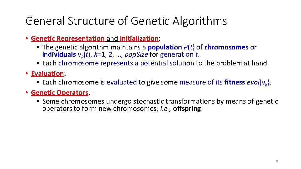
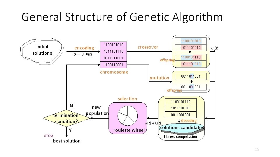
General Structure of Genetic Algorithms • Genetic Representation and Initialization: • The genetic algorithm maintains a population P(t) of chromosomes or individuals vk(t), k=1, 2, …, pop. Size for generation t. • Each chromosome represents a potential solution to the problem at hand. • Evaluation: • Each chromosome is evaluated to give some measure of its fitness eval(vk). • Genetic Operators: • Some chromosomes undergo stochastic transformations by means of genetic operators to form new chromosomes, i. e. , offspring. 8

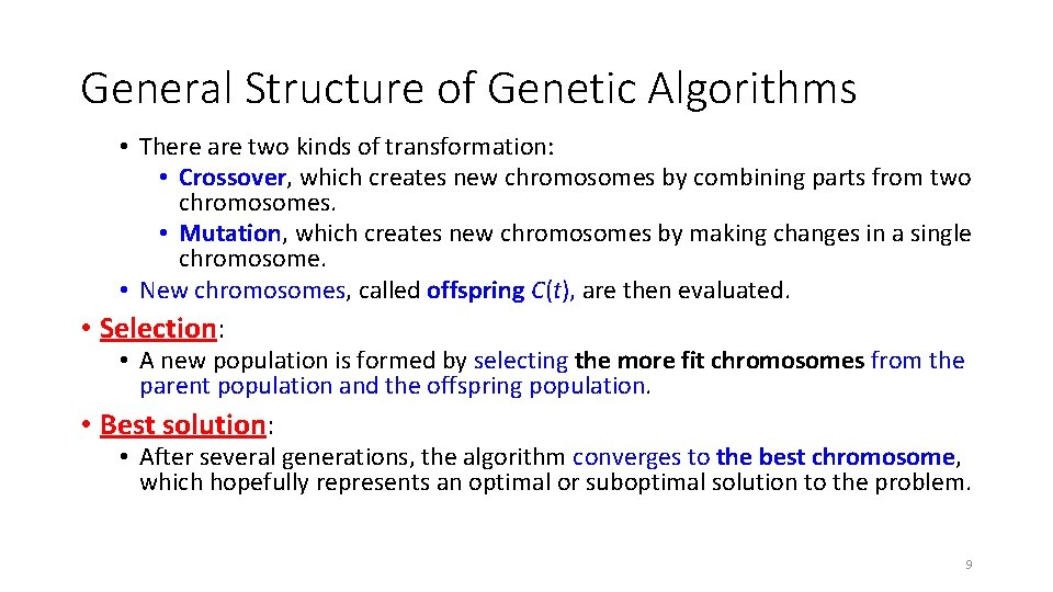
General Structure of Genetic Algorithms • There are two kinds of transformation: • Crossover, which creates new chromosomes by combining parts from two chromosomes. • Mutation, which creates new chromosomes by making changes in a single chromosome. • New chromosomes, called offspring C(t), are then evaluated. • Selection: • A new population is formed by selecting the more fit chromosomes from the parent population and the offspring population. • Best solution: • After several generations, the algorithm converges to the best chromosome, which hopefully represents an optimal or suboptimal solution to the problem. 9

General Structure of Genetic Algorithm 1100101010 Initial solutions encoding t 0 P(t) 1100101010 101110 crossover 0011011001 101110 offspring 110001 chromosome mutation CC(t) 11001011101010 0011011001 0011001001 offspring selection N termination condition? Y stop best solution 1100101110 new population 1011101010 0011001001 P(t) + C(t) roulette wheel decoding solutions candidates fitness computation 10

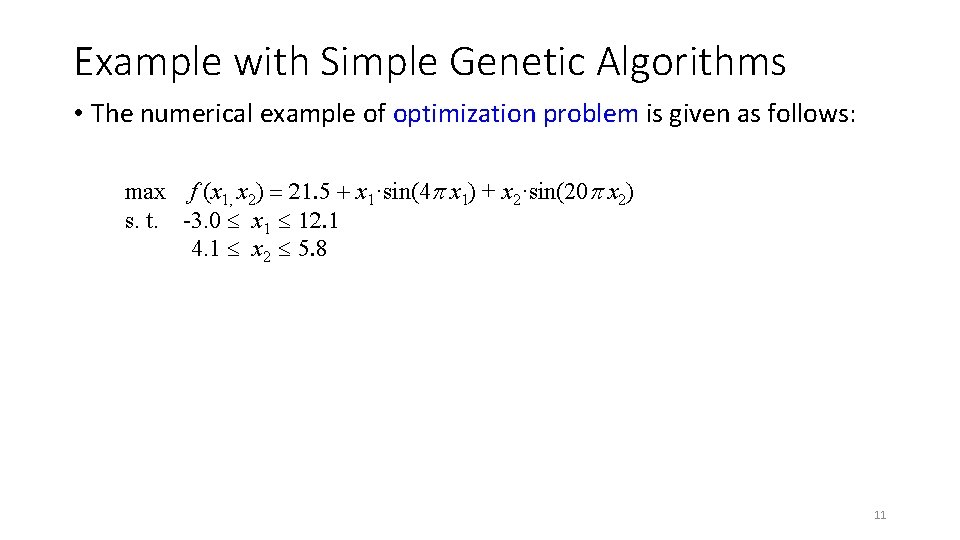
Example with Simple Genetic Algorithms • The numerical example of optimization problem is given as follows: max f (x 1, x 2) = 21. 5 + x 1·sin(4 p x 1) + x 2·sin(20 p x 2) s. t. -3. 0 x 1 12. 1 4. 1 x 2 5. 8 11

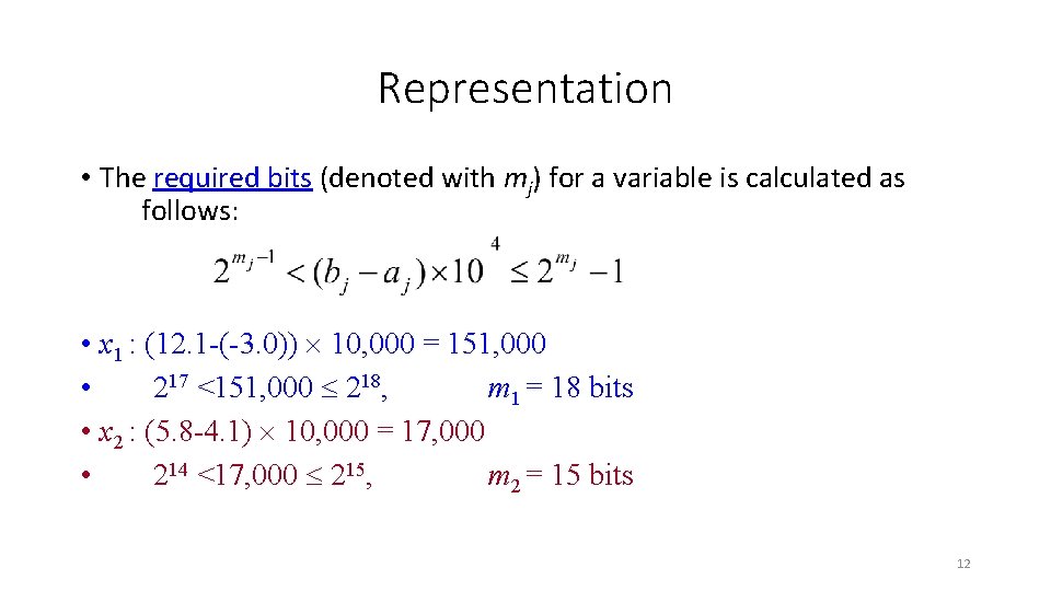
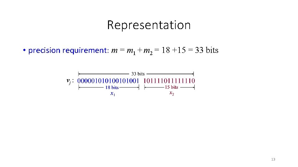
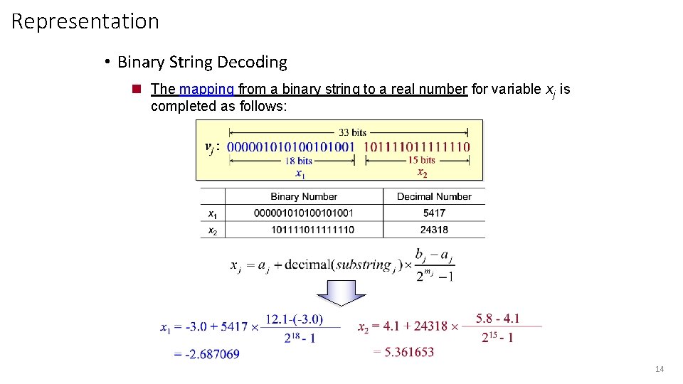
Representation • The required bits (denoted with mj) for a variable is calculated as follows: • x 1 : (12. 1 -(-3. 0)) 10, 000 = 151, 000 • 217 <151, 000 218, m 1 = 18 bits • x 2 : (5. 8 -4. 1) 10, 000 = 17, 000 • 214 <17, 000 215, m 2 = 15 bits 12

Representation • precision requirement: m = m 1 + m 2 = 18 +15 = 33 bits 13

Representation • Binary String Decoding n The mapping from a binary string to a real number for variable xj is completed as follows: 14

Initial Population • Initial population is randomly generated as follows: v 1 = [00000101010011011111110] = [x 1 x 2] = [-2. 687969 5. 361653] v 2 = [00111010111000000010101001000] = [x 1 x 2] = [ 0. 474101 4. 170144] v 3 = [111000001000010101001000110] = [x 1 x 2] = [10. 419457 4. 661461] v 4 = [1001101101000000010111001] = [x 1 x 2] = [ 6. 159951 4. 109598] v 5 = [00001011110110001110001101000] = [x 1 x 2] = [ -2. 301286 4. 477282] v 6 = [11111010101101100000001011001] = [x 1 x 2] = [11. 788084 4. 174346] v 7 = [1101001111100010011101101] = [x 1 x 2] = [ 9. 342067 5. 121702] v 8 = [00101101010000110001011001100] = [x 1 x 2] = [ -0. 330256 4. 694977] v 9 = [11111000101100011101000111101] = [x 1 x 2] = [11. 671267 4. 873501] v 10 = [111101001110100000101010] = [x 1 x 2] = [11. 446273 4. 171908] 15

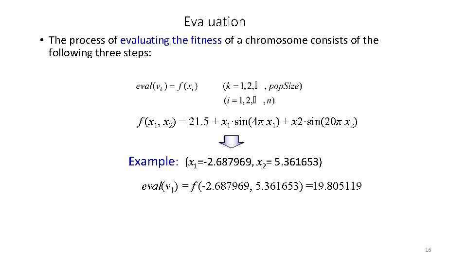
Evaluation • The process of evaluating the fitness of a chromosome consists of the following three steps: f (x 1, x 2) = 21. 5 + x 1·sin(4π x 1) + x 2·sin(20π x 2) Example: (x 1=-2. 687969, x 2= 5. 361653) eval(v 1) = f (-2. 687969, 5. 361653) =19. 805119 16

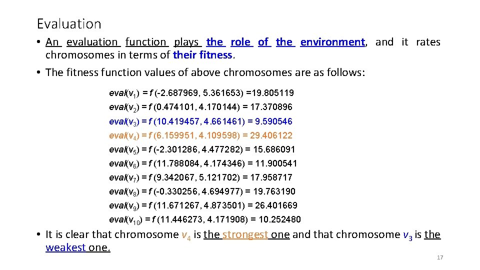
Evaluation • An evaluation function plays the role of the environment, and it rates chromosomes in terms of their fitness. • The fitness function values of above chromosomes are as follows: eval(v 1) = f (-2. 687969, 5. 361653) =19. 805119 eval(v 2) = f (0. 474101, 4. 170144) = 17. 370896 eval(v 3) = f (10. 419457, 4. 661461) = 9. 590546 eval(v 4) = f (6. 159951, 4. 109598) = 29. 406122 eval(v 5) = f (-2. 301286, 4. 477282) = 15. 686091 eval(v 6) = f (11. 788084, 4. 174346) = 11. 900541 eval(v 7) = f (9. 342067, 5. 121702) = 17. 958717 eval(v 8) = f (-0. 330256, 4. 694977) = 19. 763190 eval(v 9) = f (11. 671267, 4. 873501) = 26. 401669 eval(v 10) = f (11. 446273, 4. 171908) = 10. 252480 • It is clear that chromosome v 4 is the strongest one and that chromosome v 3 is the weakest one. 17

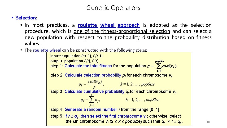
Genetic Operators • Selection: • In most practices, a roulette wheel approach is adopted as the selection procedure, which is one of the fitness-proportional selection and can select a new population with respect to the probability distribution based on fitness values. • The roulette wheel can be constructed with the following steps: input: population P(t-1), C(t-1) output: population P(t), C(t) step 1: Calculate the total fitness for the population step 2: Calculate selection probability pk for each chromosome vk step 3: Calculate cumulative probability qk for each chromosome vk step 4: Generate a random number r from the range [0, 1]. step 5: If r q 1, then select the first chromosome v 1; otherwise, select the kth chromosome vk (2 k pop. Size) such that qk-1< r qk. 18

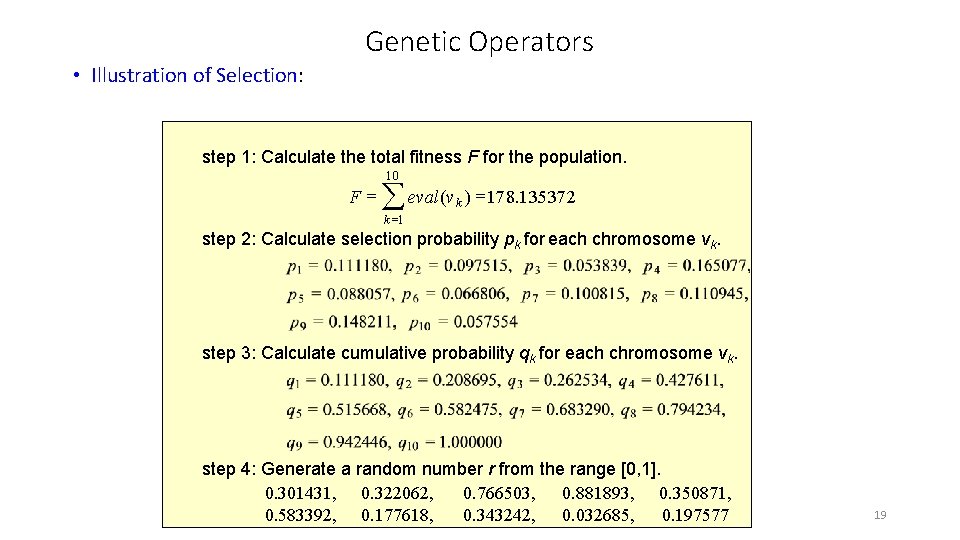
Genetic Operators • Illustration of Selection: step 1: Calculate the total fitness F for the population. F= 10 å eval(v k) =178. 135372 k =1 step 2: Calculate selection probability pk for each chromosome vk. step 3: Calculate cumulative probability qk for each chromosome vk. step 4: Generate a random number r from the range [0, 1]. 0. 301431, 0. 322062, 0. 766503, 0. 881893, 0. 350871, 0. 583392, 0. 177618, 0. 343242, 0. 032685, 0. 197577 19

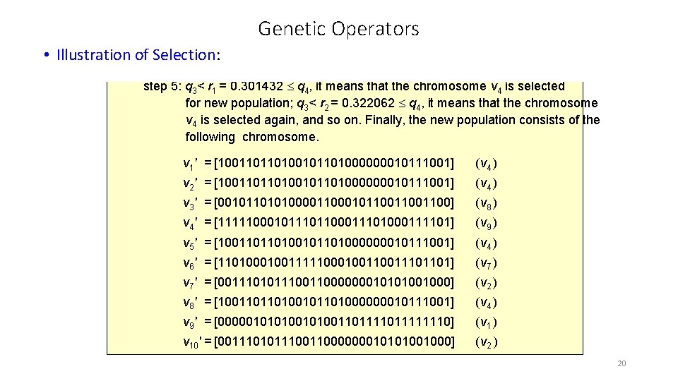
Genetic Operators • Illustration of Selection: step 5: q 3< r 1 = 0. 301432 q 4, it means that the chromosome v 4 is selected for new population; q 3< r 2 = 0. 322062 q 4, it means that the chromosome v 4 is selected again, and so on. Finally, the new population consists of the following chromosome. v 1' = [1001101101000000010111001] (v 4 ) v 2' = [1001101101000000010111001] (v 4 ) v 3' = [00101101010000110001011001100] (v 8 ) v 4' = [11111000101100011101000111101] (v 9 ) v 5' = [1001101101000000010111001] (v 4 ) v 6' = [1101001111100010011101101] (v 7 ) v 7' = [00111010111000000010101001000] (v 2 ) v 8' = [1001101101000000010111001] (v 4 ) v 9' = [00000101010011011111110] (v 1 ) v 10' = [00111010111000000010101001000] (v 2 ) 20

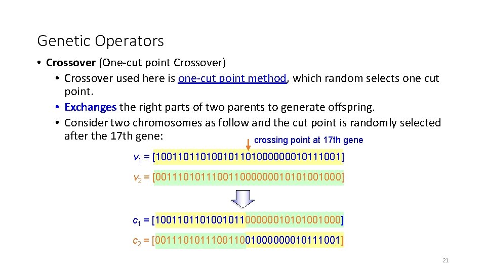
Genetic Operators • Crossover (One-cut point Crossover) • Crossover used here is one-cut point method, which random selects one cut point. • Exchanges the right parts of two parents to generate offspring. • Consider two chromosomes as follow and the cut point is randomly selected after the 17 th gene: crossing point at 17 th gene v 1 = [1001101101000000010111001] v 2 = [00111010111000000010101001000] c 1 = [100110110100101100000010101001000] c 2 = [00111010111001000000010111001] 21

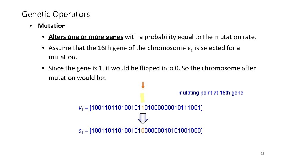
Genetic Operators • Mutation • Alters one or more genes with a probability equal to the mutation rate. • Assume that the 16 th gene of the chromosome v 1 is selected for a mutation. • Since the gene is 1, it would be flipped into 0. So the chromosome after mutation would be: mutating point at 16 th gene v 1 = [1001101101000000010111001] c 1 = [1001101101000000010101001000] 22

Example with Simple Genetic Algorithms • Next Generation v 1' = [1001101101000000010111001], f (6. 159951, 4. 109598) = 29. 406122 v 2' = [1001101101000000010111001], f (6. 159951, 4. 109598) = 29. 406122 v 3' = [00101101010000110001011001100], f (-0. 330256, 4. 694977) = 19. 763190 v 4' = [11111000101100011101000111101], f (11. 907206, 4. 873501) = 5. 702781 v 5' = [1001101101000000010111001], f (8. 024130, 4. 170248) = 19. 91025 v 6' = [1101001111100010011101101], f (9. 34067, 5. 121702) = 17. 958717 v 7' = [1001101101000000010111001], f (6. 159951, 4. 109598) = 29. 406122 v 8' = [1001101101000000010111001], f (6. 159951, 4. 109598) = 29. 406122 v 9' = [00000101010011011111110], f (-2. 687969, 5. 361653) = 19. 805199 v 10' = [00111010111000000010101001000], f (0. 474101, 4. 170248) = 17. 370896 23

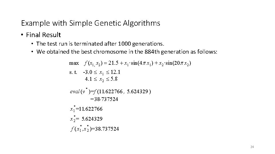
Example with Simple Genetic Algorithms • Final Result • The test run is terminated after 1000 generations. • We obtained the best chromosome in the 884 th generation as follows: max s. t. f (x 1, x 2) = 21. 5 + x 1·sin(4 p x 1) + x 2·sin(20 p x 2) -3. 0 x 1 12. 1 4. 1 x 2 5. 8 eval (v * )=f (11. 622766 , 5. 624329 ) = 38. 737524 x 1*=11. 622766 x*2= 5. 624329 f ( x 1* , x *2 )=38. 737524 24

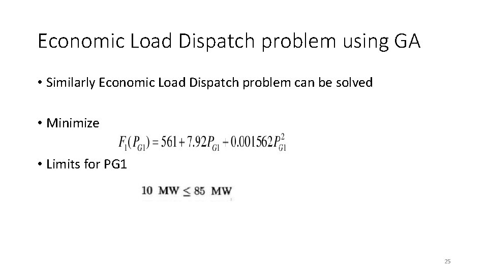
Economic Load Dispatch problem using GA • Similarly Economic Load Dispatch problem can be solved • Minimize • Limits for PG 1 25