Educational statistics 1 1 What is Statistics Statistics

Educational statistics

1. 1: What is Statistics? Statistics: The science of collecting, describing, and interpreting data. Two areas of statistics: Descriptive Statistics: collection, presentation, and description of sample data. Inferential Statistics: making decisions and drawing conclusions about populations.

Example: A college principal is interested in learning about the average of faculty. Identify the basic terms in this situation. The population is the age of all faculty members at the college. A sample is any subset of that population. For example, we might select 10 faculty members and determine their age. The variable is the “age” of each faculty member. One data would be the age of a specific faculty member. The data would be the set of values in the sample. The experiment would be the method used to select the ages forming the sample and determining the actual age of each faculty member in the sample. The parameter of interest is the “average” age of all faculty at the college. The statistic is the “average” age for all faculty in the sample.

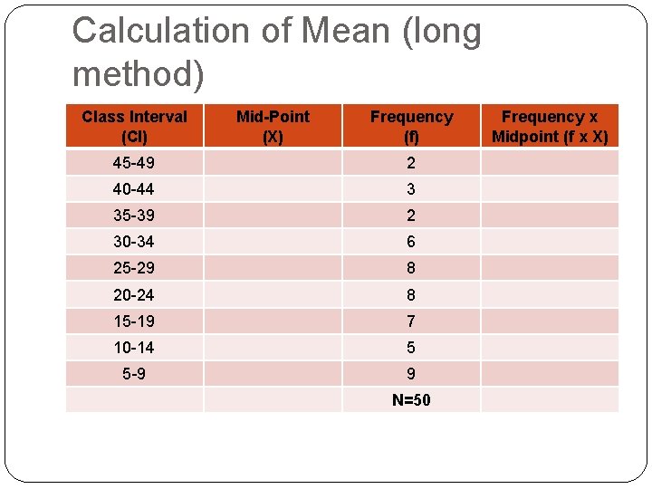
Calculation of Mean (long method) Class Interval (CI) Mid-Point (X) Frequency (f) 45 -49 2 40 -44 3 35 -39 2 30 -34 6 25 -29 8 20 -24 8 15 -19 7 10 -14 5 5 -9 9 N=50 Frequency x Midpoint (f x X)

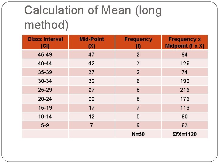
Calculation of Mean (long method) Class Interval (CI) Mid-Point (X) Frequency (f) Frequency x Midpoint (f x X) 45 -49 47 2 94 40 -44 42 3 126 35 -39 37 2 74 30 -34 32 6 192 25 -29 27 8 216 20 -24 22 8 176 15 -19 17 7 119 10 -14 12 5 60 5 -9 7 9 63 N=50 Σf. X=1120

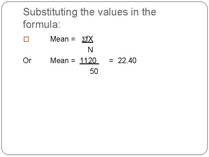
Substituting the values in the formula: � Or Mean = Σf. X N Mean = 1120 50 = 22. 40

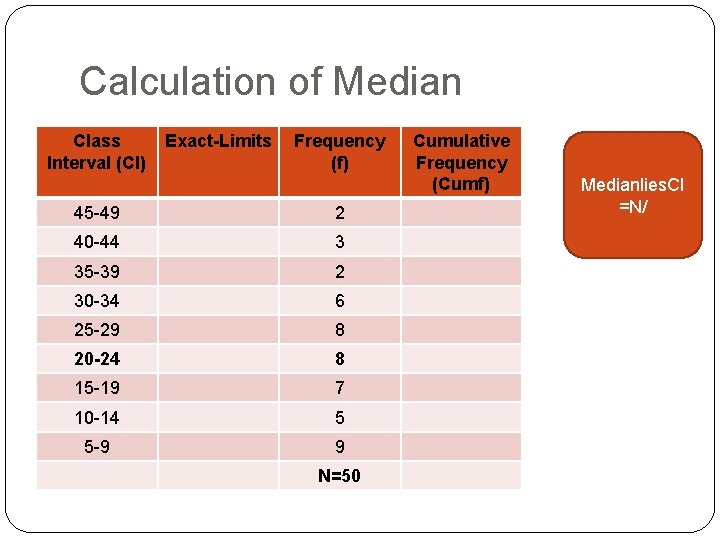
Calculation of Median Class Interval (CI) Exact-Limits Frequency (f) 45 -49 2 40 -44 3 35 -39 2 30 -34 6 25 -29 8 20 -24 8 15 -19 7 10 -14 5 5 -9 9 N=50 Cumulative Frequency (Cumf) Medianlies. CI =N/

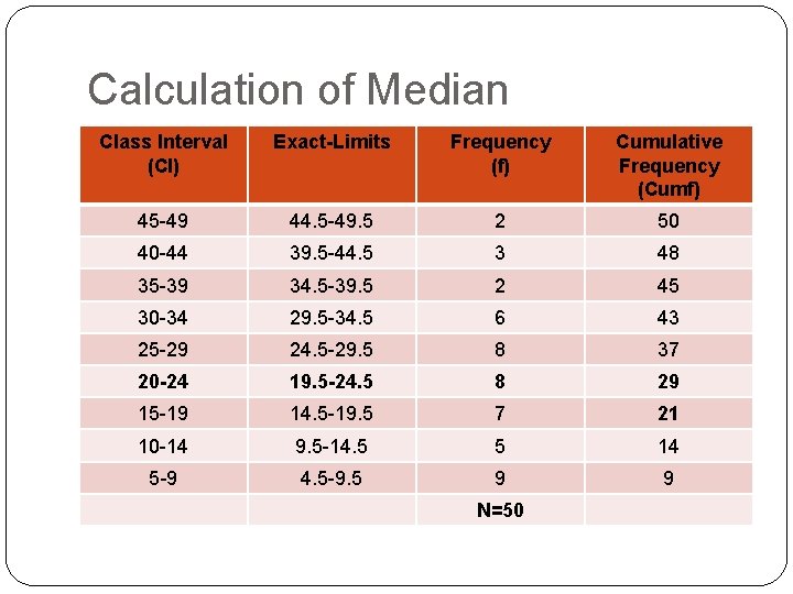
Calculation of Median Class Interval (CI) Exact-Limits Frequency (f) Cumulative Frequency (Cumf) 45 -49 44. 5 -49. 5 2 50 40 -44 39. 5 -44. 5 3 48 35 -39 34. 5 -39. 5 2 45 30 -34 29. 5 -34. 5 6 43 25 -29 24. 5 -29. 5 8 37 20 -24 19. 5 -24. 5 8 29 15 -19 14. 5 -19. 5 7 21 10 -14 9. 5 -14. 5 5 14 5 -9 4. 5 -9. 5 9 9 N=50

Substituting the values in the formula: � Median = L + [N/2 –Cumfb] x i fw L = exact lower limit of the C I in which the median lies (19. 5) Cumfb= cumulative frequency below the C I containing Median (21) fw = frequency within the C I containing the Median (8) i = size of the C I (5)

�Median = 19. 5 + [ 50/2 – 21 ] x 5 � � 8 = 19. 5 + [ 25 – 21 ] x 5 8 = 19. 5 + 4 x 5 8 = 19. 5 + 2. 5 = 22

Mode �The Mode refers to the number that occurs the most frequently. �It’s easy to remember… the first two numbers are the same! MOde and MOst Frequently!

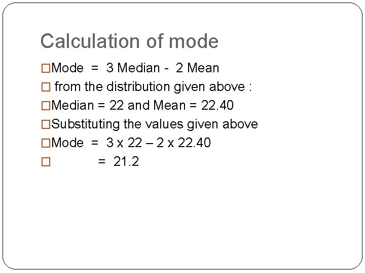
Calculation of mode �Mode = 3 Median - 2 Mean � from the distribution given above : �Median = 22 and Mean = 22. 40 �Substituting the values given above �Mode = 3 x 22 – 2 x 22. 40 � = 21. 2

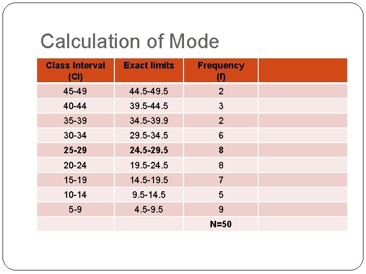
Calculation of Mode Class Interval (CI) Exact limits Frequency (f) 45 -49 44. 5 -49. 5 2 40 -44 39. 5 -44. 5 3 35 -39 34. 5 -39. 9 2 30 -34 29. 5 -34. 5 6 25 -29 24. 5 -29. 5 8 20 -24 19. 5 -24. 5 8 15 -19 14. 5 -19. 5 7 10 -14 9. 5 -14. 5 5 5 -9 4. 5 -9. 5 9 N=50

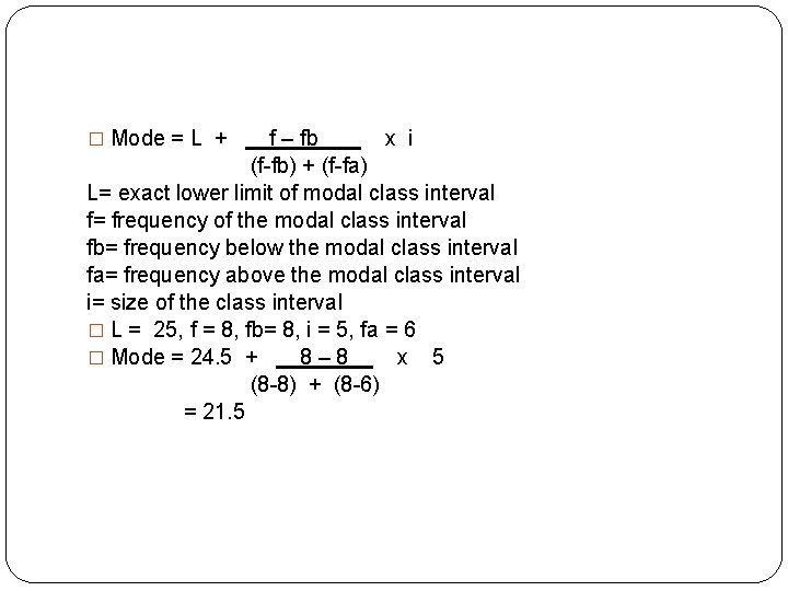
� Mode = L + f – fb x i (f-fb) + (f-fa) L= exact lower limit of modal class interval f= frequency of the modal class interval fb= frequency below the modal class interval fa= frequency above the modal class interval i= size of the class interval � L = 25, f = 8, fb= 8, i = 5, fa = 6 � Mode = 24. 5 + 8– 8 x 5 (8 -8) + (8 -6) = 21. 5

Measures of variability �Average deviation �Standard deviation �Quartile deviation

Average deviation �The average deviation is the average distance between the mean and scores in the distributions

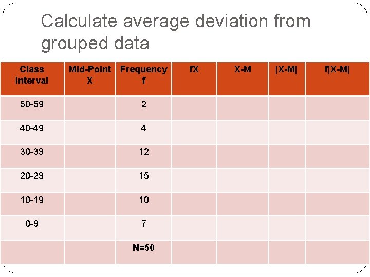
Calculate average deviation from grouped data Class interval Mid-Point X Frequency f 50 -59 2 40 -49 4 30 -39 12 20 -29 15 10 -19 10 0 -9 7 N=50 f. X X-M |X-M| f|X-M|

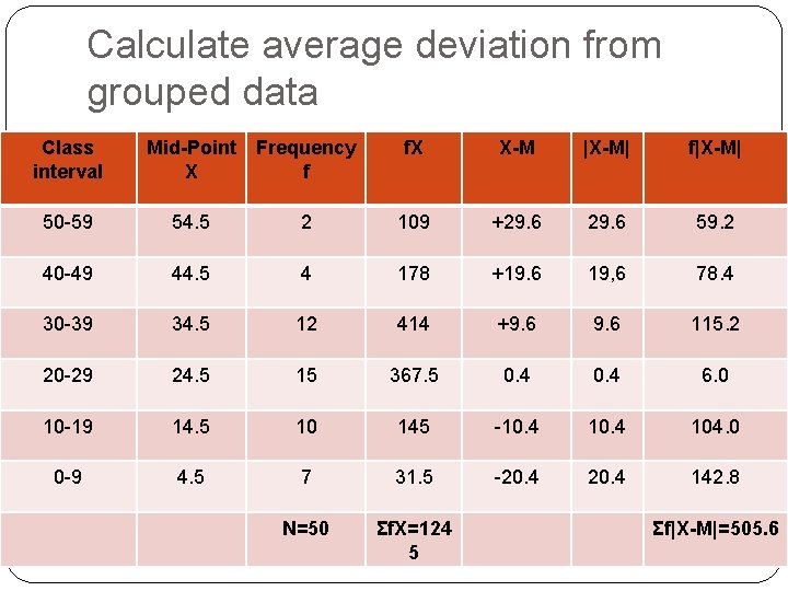
Calculate average deviation from grouped data Class interval Mid-Point X Frequency f f. X X-M |X-M| f|X-M| 50 -59 54. 5 2 109 +29. 6 59. 2 40 -49 44. 5 4 178 +19. 6 19, 6 78. 4 30 -39 34. 5 12 414 +9. 6 115. 2 20 -29 24. 5 15 367. 5 0. 4 6. 0 10 -19 14. 5 10 145 -10. 4 104. 0 0 -9 4. 5 7 31. 5 -20. 4 142. 8 N=50 Σf. X=124 5 Σf|X-M|=505. 6

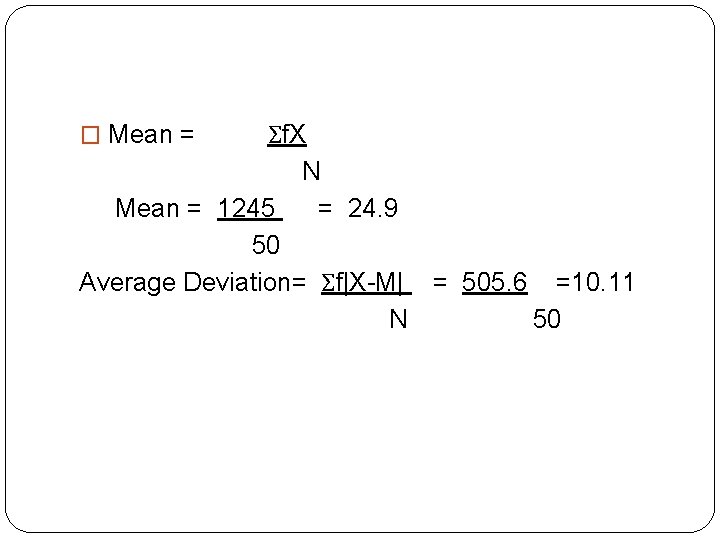
Σf. X N Mean = 1245 = 24. 9 50 Average Deviation= Σf|X-M| = 505. 6 =10. 11 N 50 � Mean =

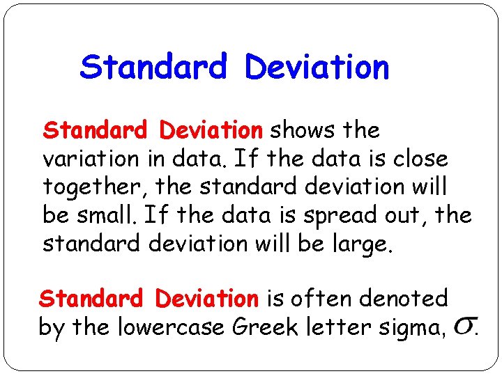
Standard Deviation shows the variation in data. If the data is close together, the standard deviation will be small. If the data is spread out, the standard deviation will be large. Standard Deviation is often denoted by the lowercase Greek letter sigma, .

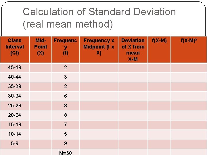
Calculation of Standard Deviation (real mean method) Class Interval (CI) Mid. Point (X) Frequenc y (f) 45 -49 2 40 -44 3 35 -39 2 30 -34 6 25 -29 8 20 -24 8 15 -19 7 10 -14 5 5 -9 9 N=50 Frequency x Midpoint (f x X) Deviation of X from mean X-M f(X-M)²

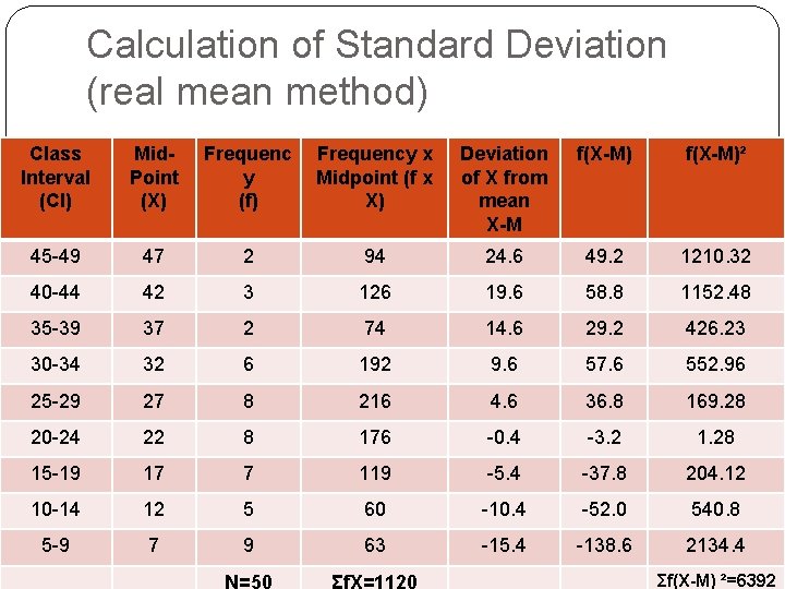
Calculation of Standard Deviation (real mean method) Class Interval (CI) Mid. Point (X) Frequenc y (f) Frequency x Midpoint (f x X) Deviation of X from mean X-M f(X-M)² 45 -49 47 2 94 24. 6 49. 2 1210. 32 40 -44 42 3 126 19. 6 58. 8 1152. 48 35 -39 37 2 74 14. 6 29. 2 426. 23 30 -34 32 6 192 9. 6 57. 6 552. 96 25 -29 27 8 216 4. 6 36. 8 169. 28 20 -24 22 8 176 -0. 4 -3. 2 1. 28 15 -19 17 7 119 -5. 4 -37. 8 204. 12 10 -14 12 5 60 -10. 4 -52. 0 540. 8 5 -9 7 9 63 -15. 4 -138. 6 2134. 4 N=50 Σf. X=1120 Σf(X-M) ²=6392

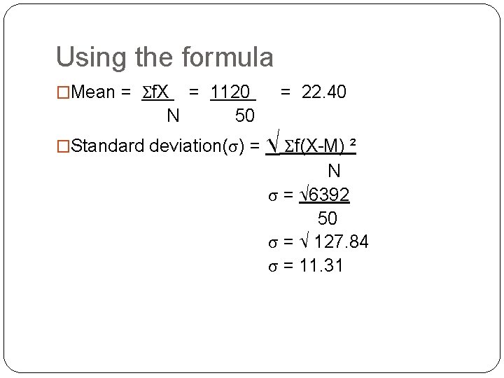
Using the formula �Mean = Σf. X = 1120 N 50 �Standard deviation(σ) = = 22. 40 √ Σf(X-M) ² N σ = √ 6392 50 σ = √ 127. 84 σ = 11. 31

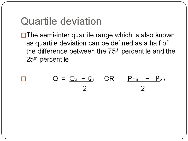
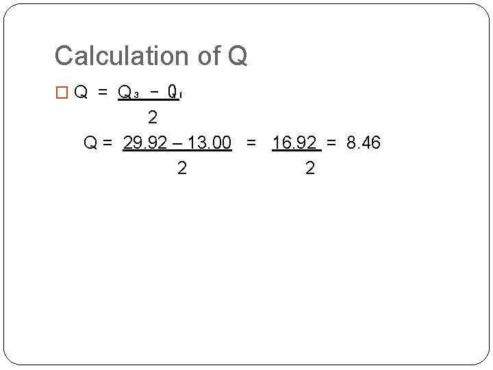
Quartile deviation �The semi-inter quartile range which is also known as quartile deviation can be defined as a half of the difference between the 75 th percentile and the 25 th percentile � Q = Q₃ - Q₁ 2 OR P₇₅ 2 P₂₅

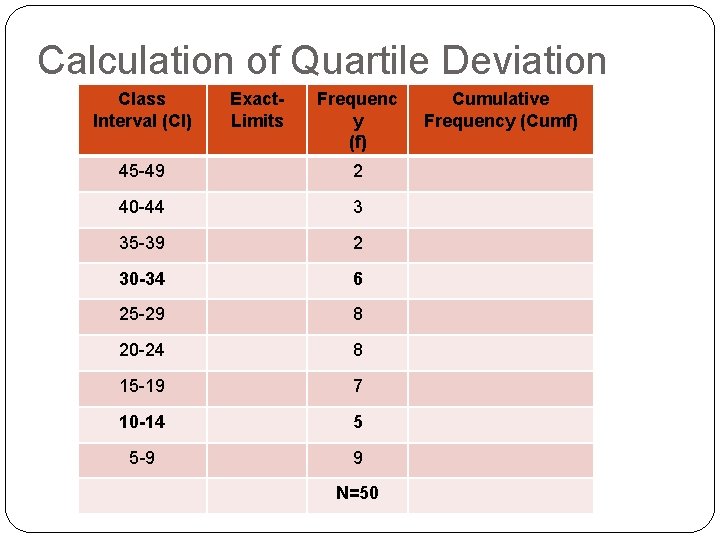
Calculation of Quartile Deviation Class Interval (CI) Exact. Limits Frequenc y (f) 45 -49 2 40 -44 3 35 -39 2 30 -34 6 25 -29 8 20 -24 8 15 -19 7 10 -14 5 5 -9 9 N=50 Cumulative Frequency (Cumf)

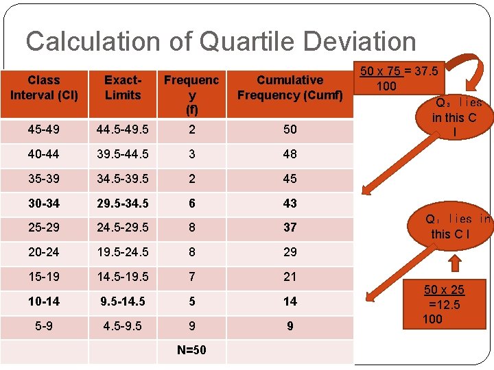
Calculation of Quartile Deviation Class Interval (CI) Exact. Limits Frequenc y (f) Cumulative Frequency (Cumf) 45 -49 44. 5 -49. 5 2 50 40 -44 39. 5 -44. 5 3 48 35 -39 34. 5 -39. 5 2 45 30 -34 29. 5 -34. 5 6 43 25 -29 24. 5 -29. 5 8 37 20 -24 19. 5 -24. 5 8 29 15 -19 14. 5 -19. 5 7 21 10 -14 9. 5 -14. 5 5 14 5 -9 4. 5 -9. 5 9 9 N=50 50 x 75 = 37. 5 100 Q₃ lies in this C I Q₁ lies in this C I 50 x 25 =12. 5 100

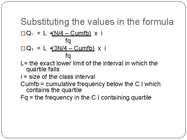
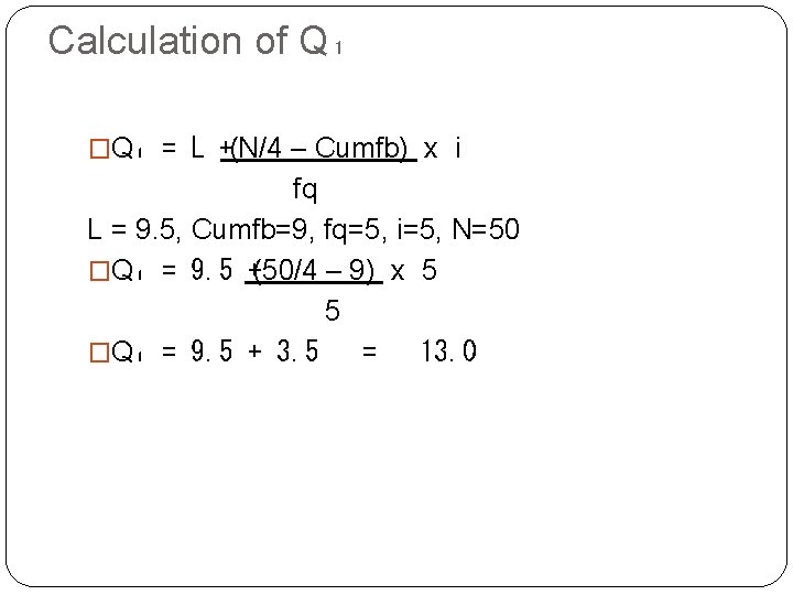
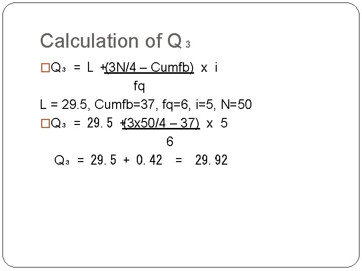
Substituting the values in the formula � Q₁ = L +(N/4 – Cumfb) x i fq � Q₃ = L +(3 N/4 – Cumfb) x i fq L= the exact lower limit of the interval in which the quartile falls i = size of the class interval Cumfb = cumulative frequency below the C I which contains the quartile Fq = the frequency in the C I containing quartile

Calculation of Q₁ �Q₁ = L +(N/4 – Cumfb) x i fq L = 9. 5, Cumfb=9, fq=5, i=5, N=50 �Q₁ = 9. 5 +(50/4 – 9) x 5 5 �Q₁ = 9. 5 + 3. 5 = 13. 0

Calculation of Q₃ �Q₃ = L +(3 N/4 – Cumfb) x i fq L = 29. 5, Cumfb=37, fq=6, i=5, N=50 �Q₃ = 29. 5 +(3 x 50/4 – 37) x 5 6 Q₃ = 29. 5 + 0. 42 = 29. 92

Calculation of Q � Q = Q₃ - Q₁ 2 Q = 29. 92 – 13. 00 = 16. 92 = 8. 46 2 2

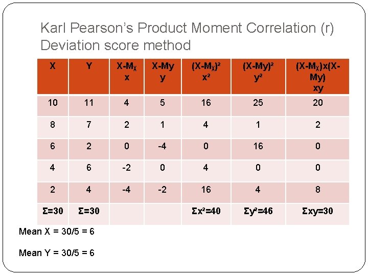
Coefficient of correlation �A Coefficient of correlation is a single number that tells us to what extent two variables or things are related and to what extent variations in one variable go with variations in the other

Karl Pearson’s Product Moment Correlation (r) Deviation score method X Y X-Mᵪ x X-My y (X-Mᵪ)² x² (X-My)² y² (X-Mᵪ)x(XMy) xy 10 11 4 5 16 25 20 8 7 2 1 4 1 2 6 2 0 -4 0 16 0 4 6 -2 0 4 0 0 2 4 -4 -2 16 4 8 Σ=30 Σx²=40 Σy²=46 Σxy=30 Mean X = 30/5 = 6 Mean Y = 30/5 = 6

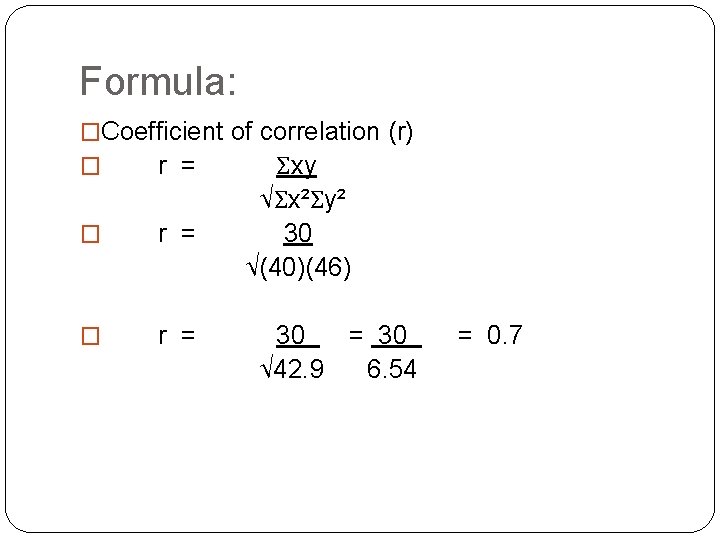
Formula: �Coefficient of correlation (r) � r = Σxy � r = √Σx²Σy² 30 √(40)(46) 30 = 30 √ 42. 9 6. 54 = 0. 7

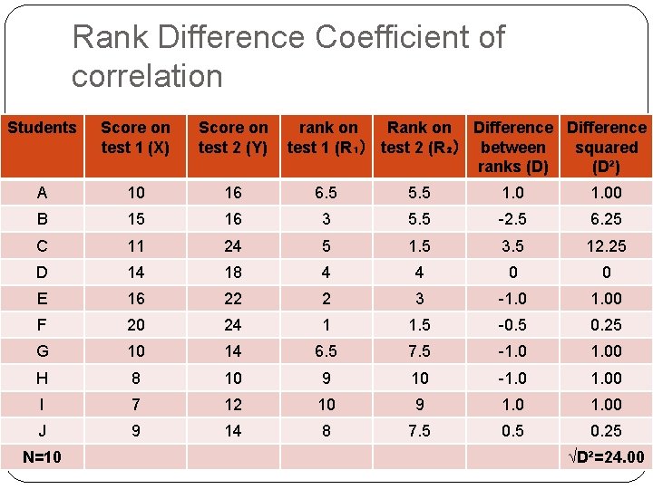
Rank Difference Coefficient of correlation Students Score on test 1 (X) Score on test 2 (Y) A 10 16 6. 5 5. 5 1. 00 B 15 16 3 5. 5 -2. 5 6. 25 C 11 24 5 1. 5 3. 5 12. 25 D 14 18 4 4 0 0 E 16 22 2 3 -1. 00 F 20 24 1 1. 5 -0. 5 0. 25 G 10 14 6. 5 7. 5 -1. 00 H 8 10 9 10 -1. 00 I 7 12 10 9 1. 00 J 9 14 8 7. 5 0. 25 N=10 rank on Rank on Difference test 1 (R₁) test 2 (R₂) between squared ranks (D) (D²) √D²=24. 00

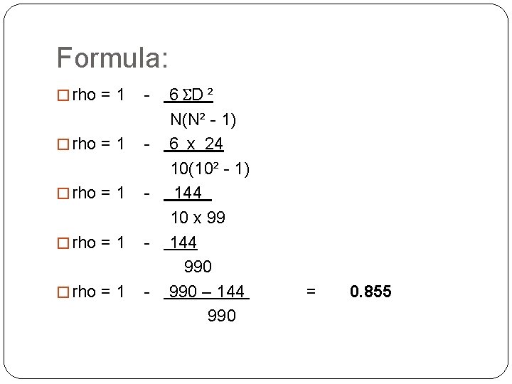
Formula: � rho = 1 - � rho = 1 - 6 ΣD ² N(N² - 1) 6 x 24 10(10² - 1) 144 10 x 99 144 990 – 144 990 = 0. 855