EDU 702 RESEARCH METHODOLOGY Presented by NORAZLIYATI YAHYA
EDU 702 RESEARCH METHODOLOGY Presented by : NORAZLIYATI YAHYA NURHARANI SELAMAT NUR HAFIZA NGADENIN 2009905123 2009324059 2009720649
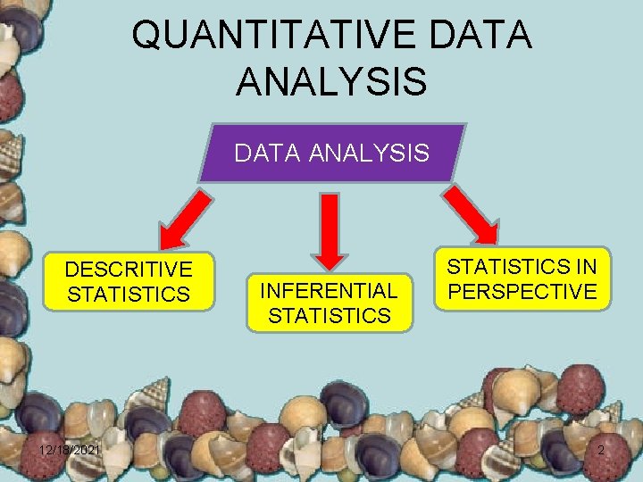
QUANTITATIVE DATA ANALYSIS DESCRITIVE STATISTICS 12/18/2021 INFERENTIAL STATISTICS IN PERSPECTIVE 2
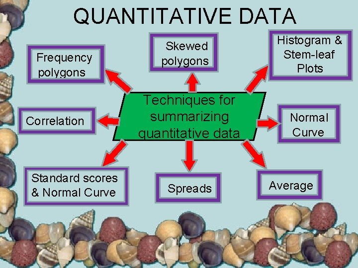
QUANTITATIVE DATA Frequency polygons Correlation Standard scores & Normal Curve Skewed polygons Techniques for summarizing quantitative data Spreads Histogram & Stem-leaf Plots Normal Curve Average
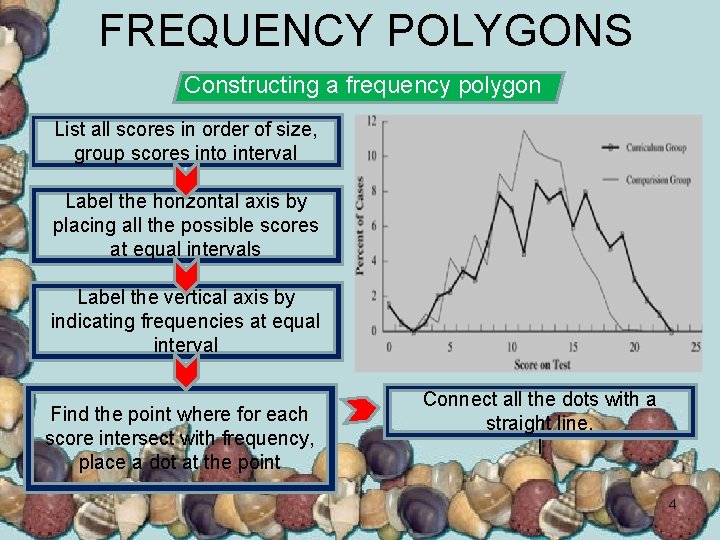
FREQUENCY POLYGONS Constructing a frequency polygon List all scores in order of size, group scores into interval Label the horizontal axis by placing all the possible scores at equal intervals Label the vertical axis by indicating frequencies at equal interval Find the point where for each score intersect with frequency, place a dot at the point Connect all the dots with a straight line. l 4
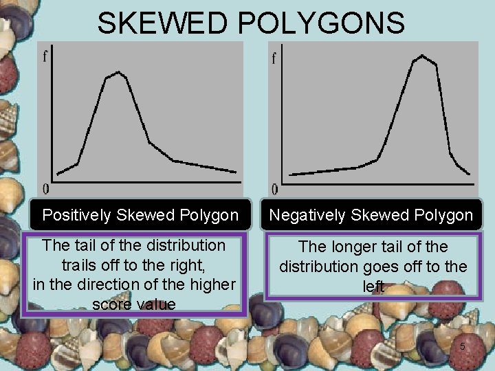
SKEWED POLYGONS Positively Skewed Polygon The tail of the distribution trails off to the right, in the direction of the higher score value Negatively Skewed Polygon The longer tail of the distribution goes off to the left 5
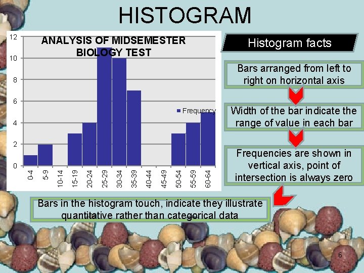
HISTOGRAM 12 ANALYSIS OF MIDSEMESTER BIOLOGY TEST 10 Histogram facts Bars arranged from left to right on horizontal axis 8 6 Frequency 4 2 60 -64 55 -59 50 -54 45 -49 40 -44 35 -39 30 -34 25 -29 20 -24 15 -19 10 -14 5 -9 0 -4 0 Width of the bar indicate the range of value in each bar Frequencies are shown in vertical axis, point of intersection is always zero Bars in the histogram touch, indicate they illustrate quantitative rather than categorical data 6
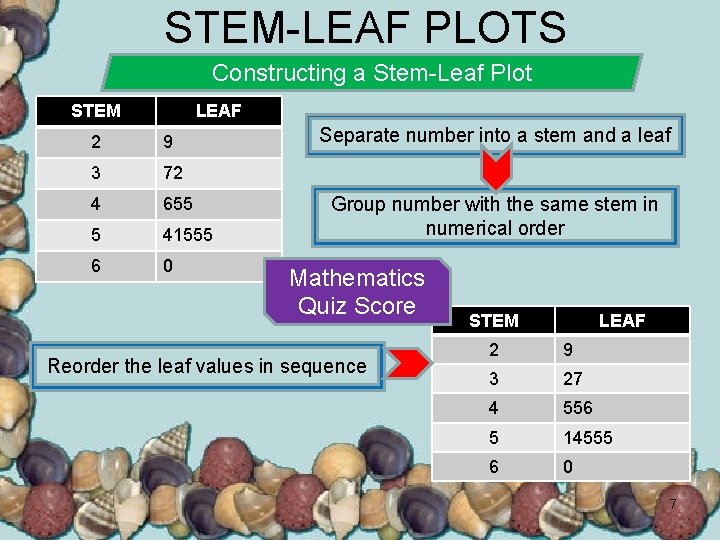
STEM-LEAF PLOTS Constructing a Stem-Leaf Plot STEM LEAF 2 9 3 72 4 655 5 41555 6 0 Separate number into a stem and a leaf Group number with the same stem in numerical order Mathematics Quiz Score Reorder the leaf values in sequence STEM LEAF 2 9 3 27 4 556 5 14555 6 0 7
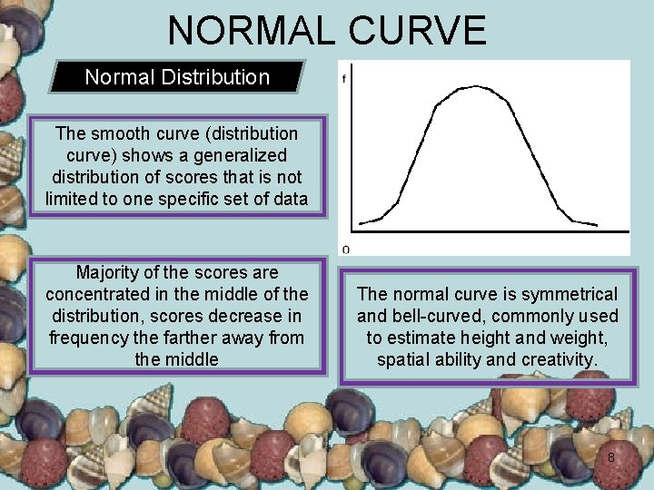
NORMAL CURVE Normal Distribution The smooth curve (distribution curve) shows a generalized distribution of scores that is not limited to one specific set of data Majority of the scores are concentrated in the middle of the distribution, scores decrease in frequency the farther away from the middle The normal curve is symmetrical and bell-curved, commonly used to estimate height and weight, spatial ability and creativity. 8
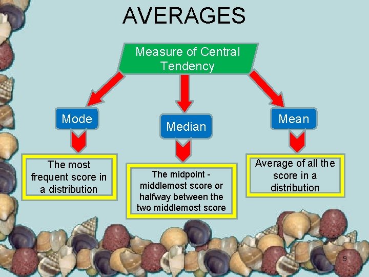
AVERAGES Measure of Central Tendency Mode The most frequent score in a distribution Median The midpoint middlemost score or halfway between the two middlemost score Mean Average of all the score in a distribution 9
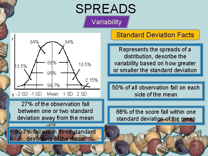
SPREADS Variability Standard Deviation Facts 34% 13. 5% 34% 68% 13. 5% 95% Represents the spreads of a distribution, describe the variability based on how greater or smaller the standard deviation 2. 15% 99. 7% -2 SD -1 SD Mean 1 SD 27% of the observation fall between one or two standard deviation away from the mean 50% of all observation fall on each side of the mean 68% of the score fall within one standard deviation of the mean 99. 7% fall within three standard deviations of the mean 10
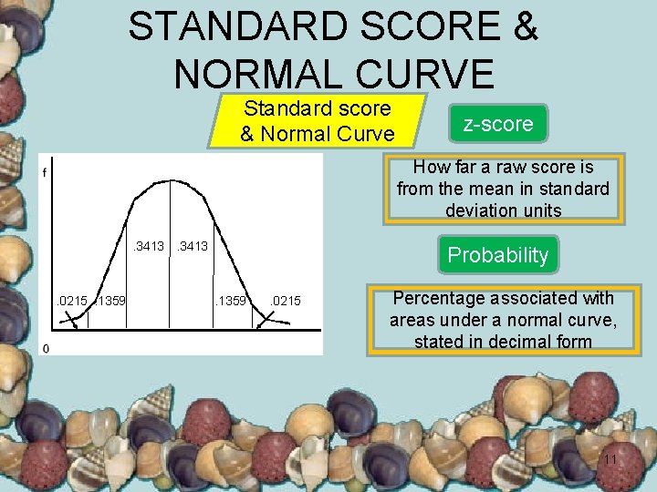
STANDARD SCORE & NORMAL CURVE Standard score & Normal Curve z-score How far a raw score is from the mean in standard deviation units . 3413 . 0215. 1359 Probability. 1359 . 0215 Percentage associated with areas under a normal curve, stated in decimal form 11
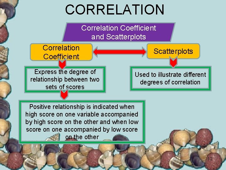
CORRELATION Correlation Coefficient and Scatterplots Correlation Coefficient Express the degree of relationship between two sets of scores Scatterplots Used to illustrate different degrees of correlation Positive relationship is indicated when high score on one variable accompanied by high score on the other and when low score on one accompanied by low score on the other 12
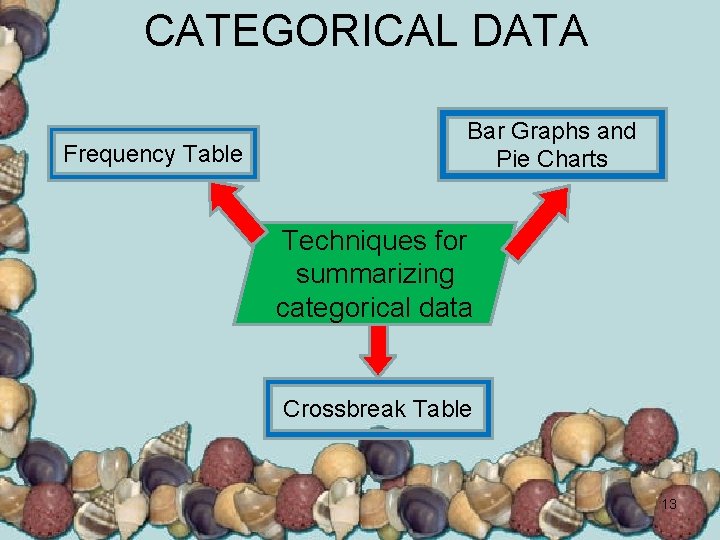
CATEGORICAL DATA Frequency Table Bar Graphs and Pie Charts Techniques for summarizing categorical data Crossbreak Table 13
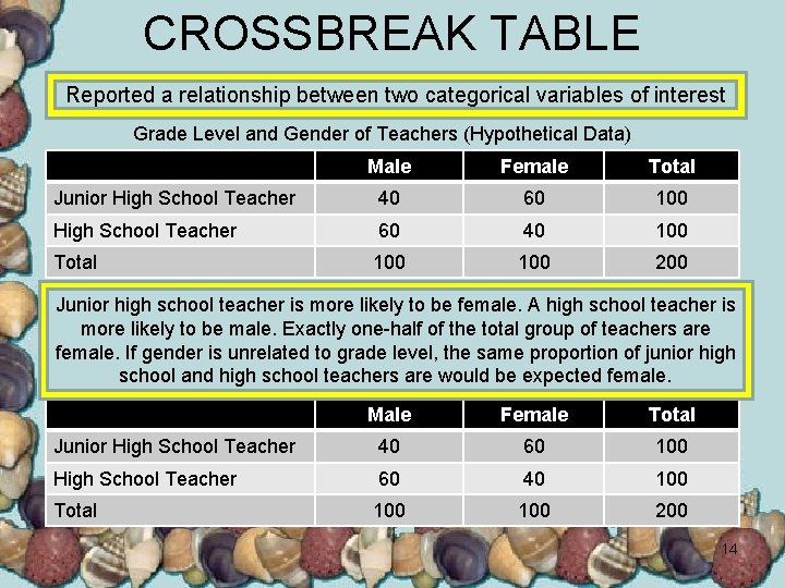
CROSSBREAK TABLE Reported a relationship between two categorical variables of interest Grade Level and Gender of Teachers (Hypothetical Data) Male Female Total Junior High School Teacher 40 60 100 High School Teacher 60 40 100 Total 100 200 Junior high school teacher is more likely to be female. A high school teacher is more likely to be male. Exactly one-half of the total group of teachers are female. If gender is unrelated to grade level, the same proportion of junior high school and high school teachers are would be expected female. Male Female Total Junior High School Teacher 40 60 100 High School Teacher 60 40 100 Total 100 200 14
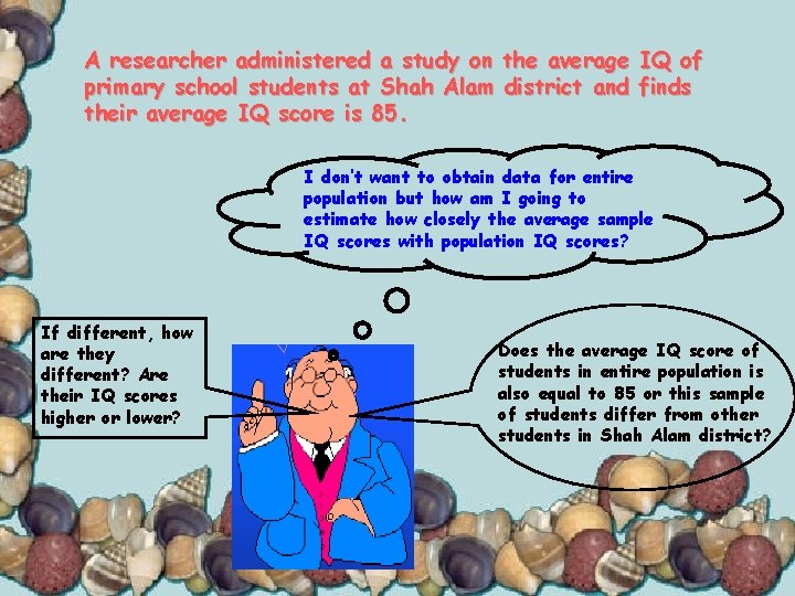
A researcher administered a study on the average IQ of primary school students at Shah Alam district and finds their average IQ score is 85. I don’t want to obtain data for entire population but how am I going to estimate how closely the average sample IQ scores with population IQ scores? If different, how are they different? Are their IQ scores higher or lower? Does the average IQ score of students in entire population is also equal to 85 or this sample of students differ from other students in Shah Alam district?
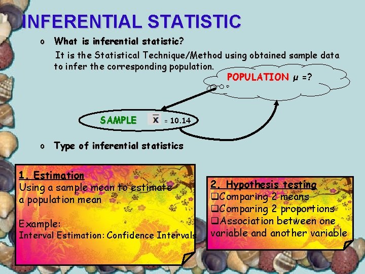
INFERENTIAL STATISTIC o What is inferential statistic? It is the Statistical Technique/Method using obtained sample data to infer the corresponding population. POPULATION μ =? SAMPLE = 10. 14 o Type of inferential statistics 1. Estimation Using a sample mean to estimate a population mean Example: Interval Estimation: Confidence Intervals 2. Hypothesis testing q. Comparing 2 means q. Comparing 2 proportions q. Association between one variable and another variable
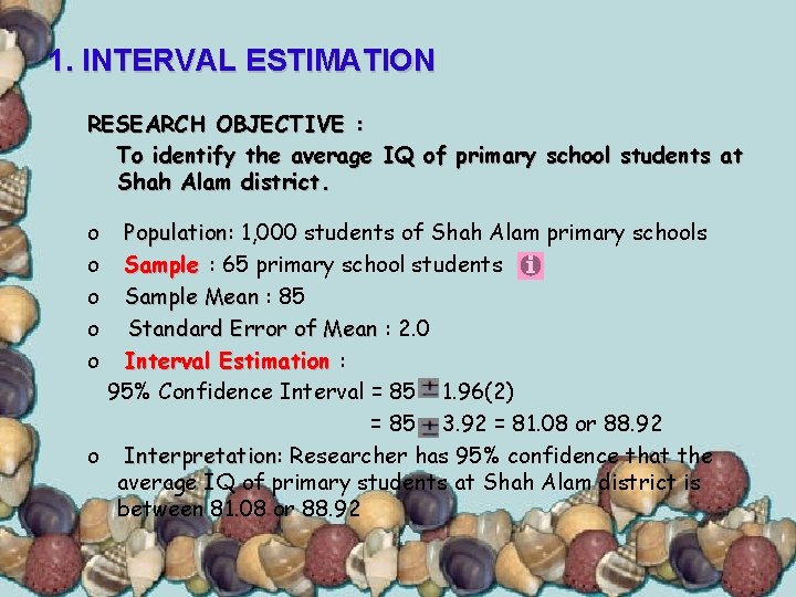
1. INTERVAL ESTIMATION RESEARCH OBJECTIVE : To identify the average IQ of primary school students at Shah Alam district. o o o Population: Population 1, 000 students of Shah Alam primary schools Sample : 65 primary school students Sample Mean : 85 Standard Error of Mean : 2. 0 Interval Estimation : 95% Confidence Interval = 85 1. 96(2) = 85 3. 92 = 81. 08 or 88. 92 o Interpretation: Interpretation Researcher has 95% confidence that the average IQ of primary students at Shah Alam district is between 81. 08 or 88. 92
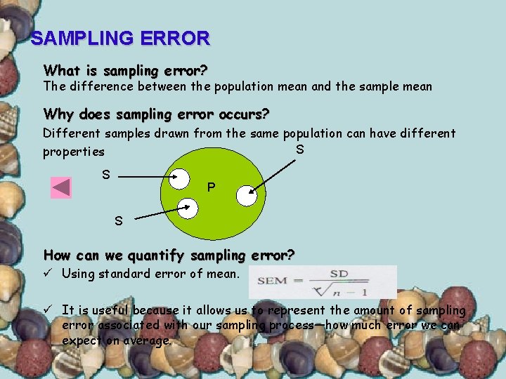
SAMPLING ERROR What is sampling error? The difference between the population mean and the sample mean Why does sampling error occurs? Different samples drawn from the same population can have different S properties S P S How can we quantify sampling error? ü Using standard error of mean. ü It is useful because it allows us to represent the amount of sampling error associated with our sampling process—how much error we can expect on average.
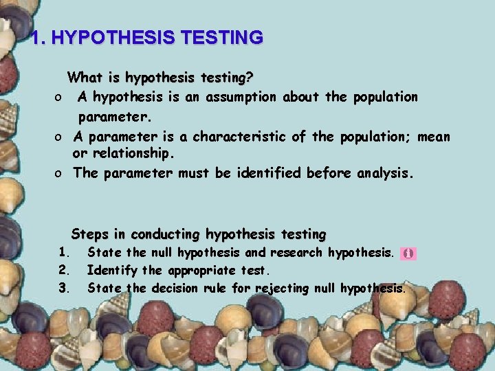
1. HYPOTHESIS TESTING What is hypothesis testing? o A hypothesis is an assumption about the population parameter. o A parameter is a characteristic of the population; mean or relationship. o The parameter must be identified before analysis. Steps in conducting hypothesis testing 1. 2. 3. State the null hypothesis and research hypothesis. Identify the appropriate test. State the decision rule for rejecting null hypothesis.
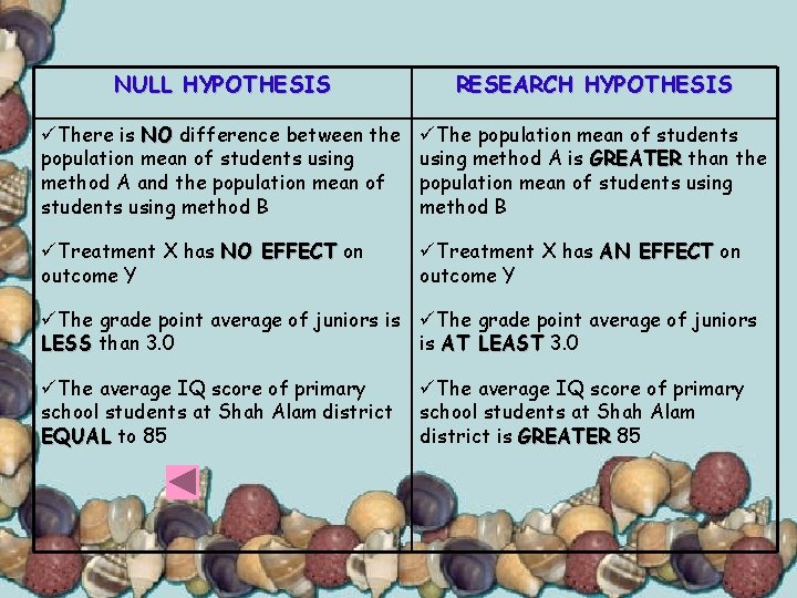
NULL HYPOTHESIS RESEARCH HYPOTHESIS üThere is NO difference between the population mean of students using method A and the population mean of students using method B üThe population mean of students using method A is GREATER than the population mean of students using method B üTreatment X has NO EFFECT on outcome Y üTreatment X has AN EFFECT on outcome Y üThe grade point average of juniors is üThe grade point average of juniors LESS than 3. 0 is AT LEAST 3. 0 üThe average IQ score of primary school students at Shah Alam district EQUAL to 85 üThe average IQ score of primary school students at Shah Alam district is GREATER 85
NULL HYPOTHESIS The average IQ score of primary school students at Shah Alam district EQUAL to 85 This test is called one sample t test. At the end of the hypothesis testing, we will get a P value. If the P value is less than 0. 05, we reject the Null Hypothesis and conclude as Research Hypothesis. § If the P value is more than or equal to 0. 05, we cannot reject the Null Hypothesis. § In above example, if we get P =0. 01, we reject the null hypothesis, then we conclude Research Hypothesis “the average IQ score of primary school students at Shah Alam district is GREATER 85 ”. § § §
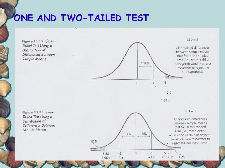
ONE AND TWO-TAILED TEST
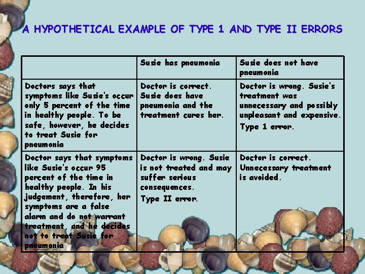
A HYPOTHETICAL EXAMPLE OF TYPE 1 AND TYPE II ERRORS Susie has pneumonia Susie does not have pneumonia Doctors says that symptoms like Susie’s occur only 5 percent of the time in healthy people. To be safe, however, he decides to treat Susie for pneumonia Doctor is correct. Susie does have pneumonia and the treatment cures her. Doctor is wrong. Susie’s treatment was unnecessary and possibly unpleasant and expensive. Type 1 error. Doctor says that symptoms like Susie’s occur 95 percent of the time in healthy people. In his judgement, therefore, her symptoms are a false alarm and do not warrant treatment, and he decides not to treat Susie for pneumonia Doctor is wrong. Susie is not treated and may suffer serious consequences. Type II error. Doctor is correct. Unnecessary treatment is avoided.
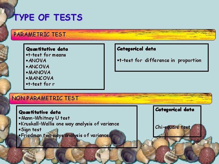
TYPE OF TESTS PARAMETRIC TEST Quantitative data §t-test for means §ANOVA §ANCOVA §MANCOVA §t-test for r Categorical data §t-test for difference in proportion NON PARAMETRIC TEST Quantitative data §Mann-Whitney U test §Kruskall-Wallis one way analysis of variance §Sign test §Friedman two ways analysis of variance Categorical data Chi-square test
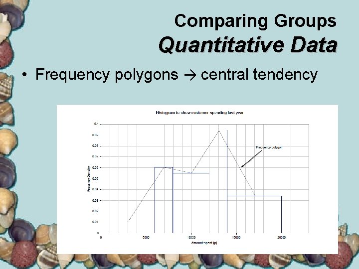
Comparing Groups Quantitative Data • Frequency polygons → central tendency
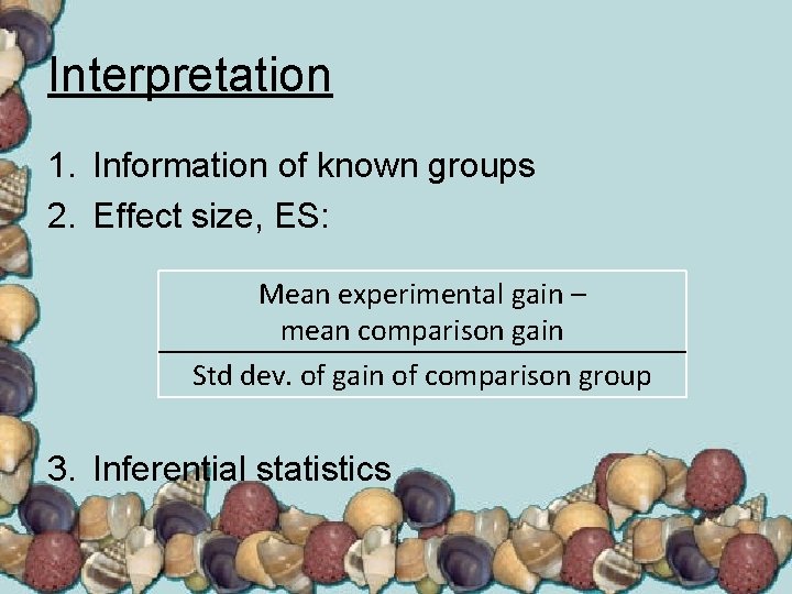
Interpretation 1. Information of known groups 2. Effect size, ES: Mean experimental gain – mean comparison gain Std dev. of gain of comparison group 3. Inferential statistics
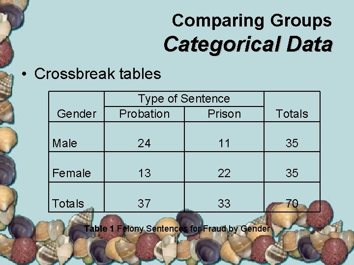
Comparing Groups Categorical Data • Crossbreak tables Gender Type of Sentence Probation Prison Totals Male 24 11 35 Female 13 22 35 Totals 37 33 70 Table 1 Felony Sentences for Fraud by Gender
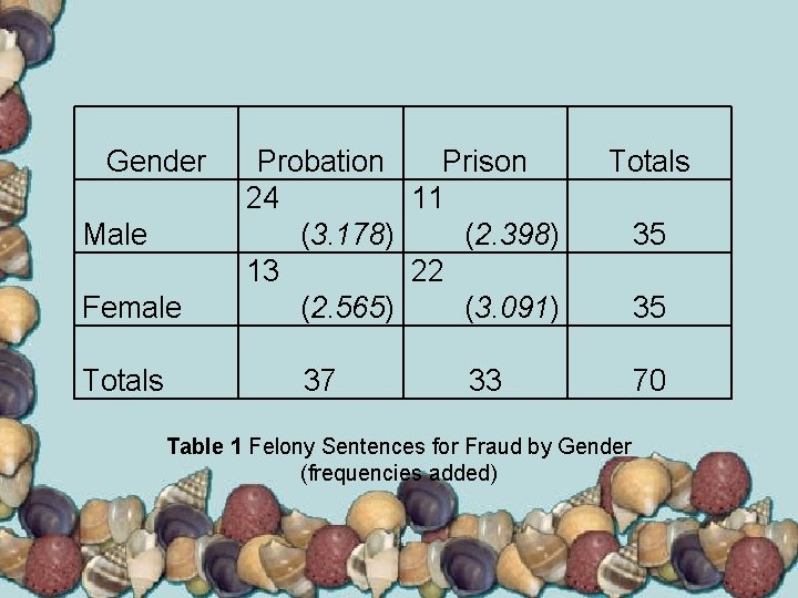
Gender Male Female Totals Probation Prison 24 11 (3. 178) (2. 398) 13 22 (2. 565) (3. 091) 37 Totals 33 Table 1 Felony Sentences for Fraud by Gender (frequencies added) 35 35 70
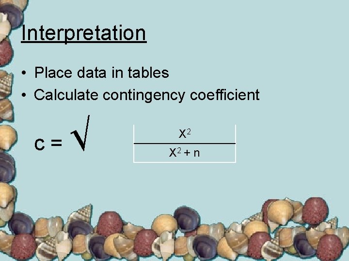
Interpretation • Place data in tables • Calculate contingency coefficient c= √ X 2 + n

THANK YOU. . .
- Slides: 30