EDP 554 AnalysisofVariance Methods Arizona State University Statistical

EDP 554 Analysis-of-Variance Methods Arizona State University Statistical Inference with Z- and t-Tests Dr. J. Bryan Henderson

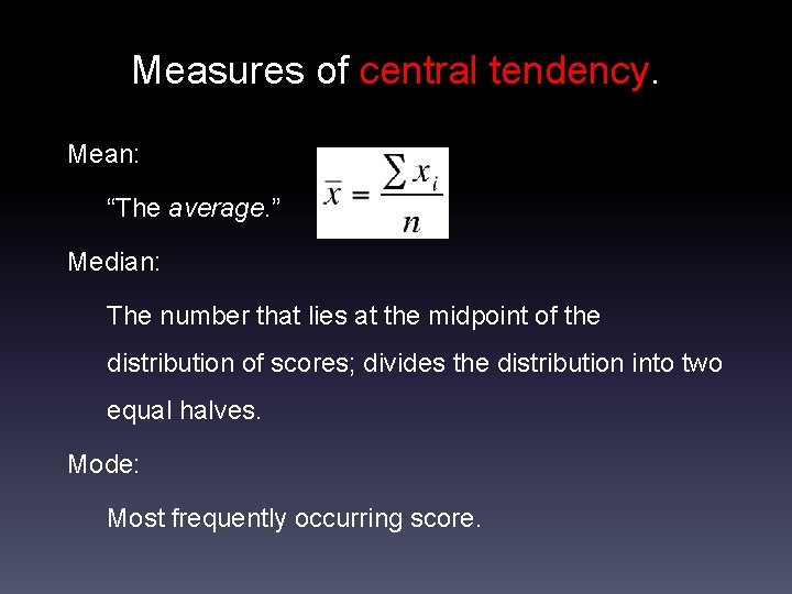
Measures of central tendency. Mean: “The average. ” Median: The number that lies at the midpoint of the distribution of scores; divides the distribution into two equal halves. Mode: Most frequently occurring score.

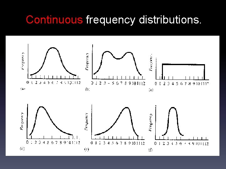
Continuous frequency distributions.

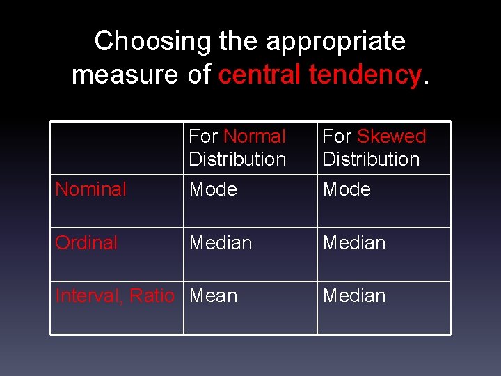
Choosing the appropriate measure of central tendency. For Normal Distribution For Skewed Distribution Nominal Mode Ordinal Median Interval, Ratio Mean Median

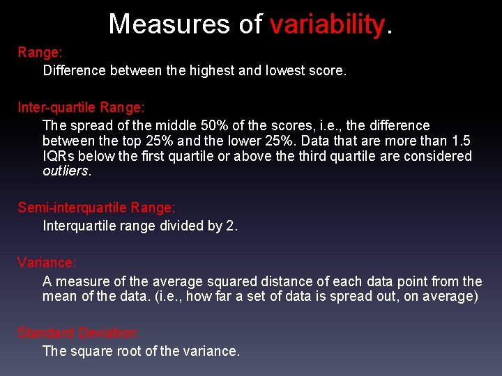
Measures of variability. Range: Difference between the highest and lowest score. Inter-quartile Range: The spread of the middle 50% of the scores, i. e. , the difference between the top 25% and the lower 25%. Data that are more than 1. 5 IQRs below the first quartile or above third quartile are considered outliers. Semi-interquartile Range: Interquartile range divided by 2. Variance: A measure of the average squared distance of each data point from the mean of the data. (i. e. , how far a set of data is spread out, on average) Standard Deviation: The square root of the variance.

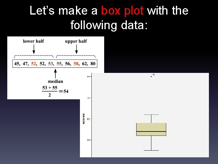
Let’s make a box plot with the following data:

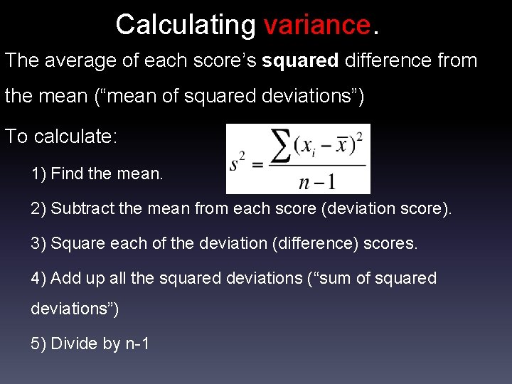
Calculating variance. The average of each score’s squared difference from the mean (“mean of squared deviations”) To calculate: 1) Find the mean. 2) Subtract the mean from each score (deviation score). 3) Square each of the deviation (difference) scores. 4) Add up all the squared deviations (“sum of squared deviations”) 5) Divide by n-1

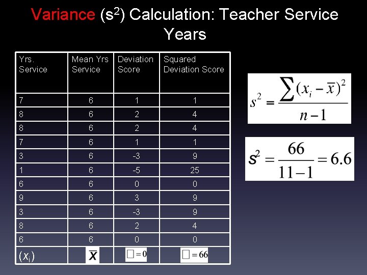
Variance (s 2) Calculation: Teacher Service Years Yrs. Service Mean Yrs Service Deviation Score Squared Deviation Score 7 6 1 1 8 6 2 4 7 6 1 1 3 6 -3 9 1 6 -5 25 6 6 0 0 9 6 3 9 3 6 -3 9 8 6 2 4 6 6 0 0 (xi)

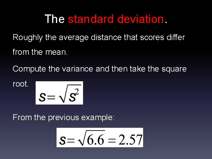
The standard deviation. Roughly the average distance that scores differ from the mean. Compute the variance and then take the square root. From the previous example:

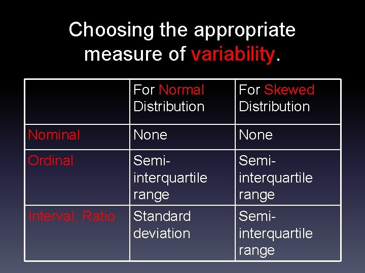
Choosing the appropriate measure of variability. For Normal Distribution For Skewed Distribution Nominal None Ordinal Semiinterquartile range Interval, Ratio Standard deviation Semiinterquartile range

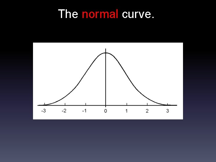
The normal curve.

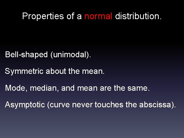
Properties of a normal distribution. Bell-shaped (unimodal). Symmetric about the mean. Mode, median, and mean are the same. Asymptotic (curve never touches the abscissa).

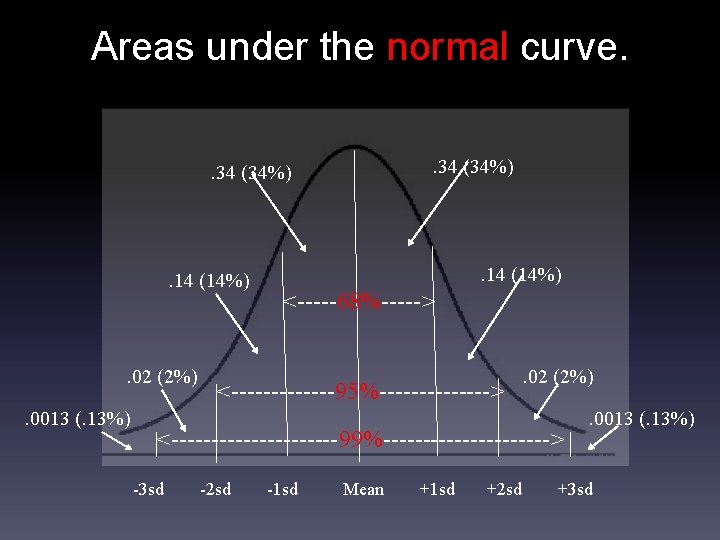
Areas under the normal curve. . 34 (34%) . 14 (14%) . 02 (2%). 0013 (. 13%) . 14 (14%) <-----68%-----> <-------95%-------> . 02 (2%) <-----------99%-----------> -3 sd -2 sd -1 sd Mean +1 sd +2 sd . 0013 (. 13%) +3 sd

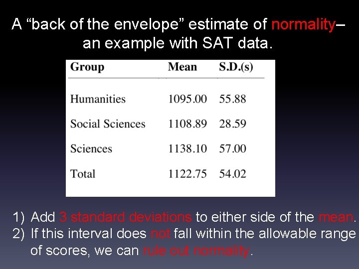
A “back of the envelope” estimate of normality– an example with SAT data. 1) Add 3 standard deviations to either side of the mean. 2) If this interval does not fall within the allowable range of scores, we can rule out normality.

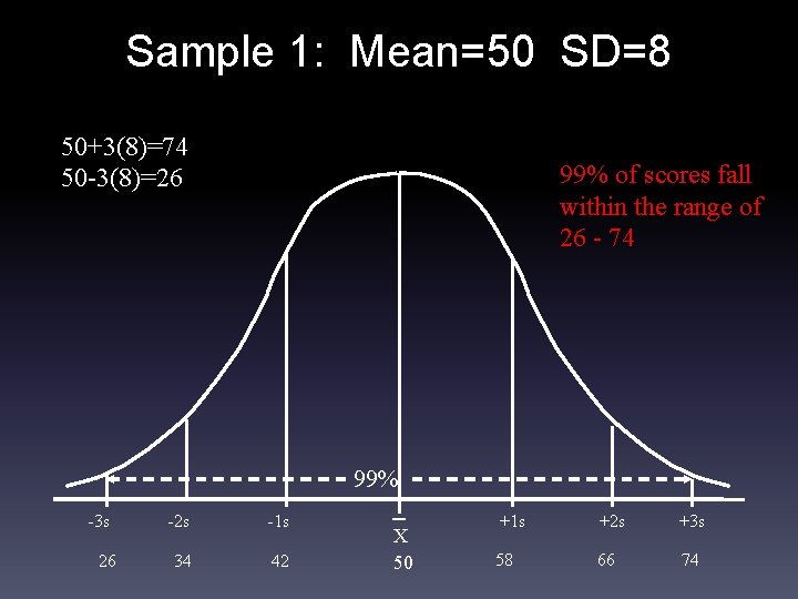
Sample 1: Mean=50 SD=8 50+3(8)=74 50 -3(8)=26 99% of scores fall within the range of 26 - 74 99% -3 s 26 -2 s -1 s 34 42 X 50 +1 s +2 s +3 s 58 66 74

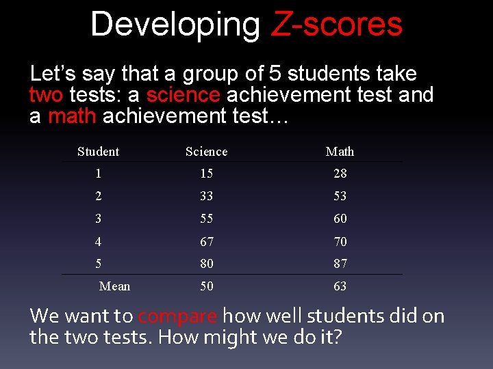
Developing Z-scores Let’s say that a group of 5 students take two tests: a science achievement test and a math achievement test… Student Science Math 1 15 28 2 33 53 3 55 60 4 67 70 5 80 87 50 63 Mean We want to compare how well students did on the two tests. How might we do it?

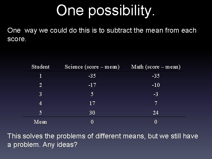
One possibility. One way we could do this is to subtract the mean from each score. Student Science (score – mean) Math (score – mean) 1 -35 2 -17 -10 3 5 -3 4 17 7 5 30 24 Mean 0 0 This solves the problems of different means, but we still have a problem. Any ideas?

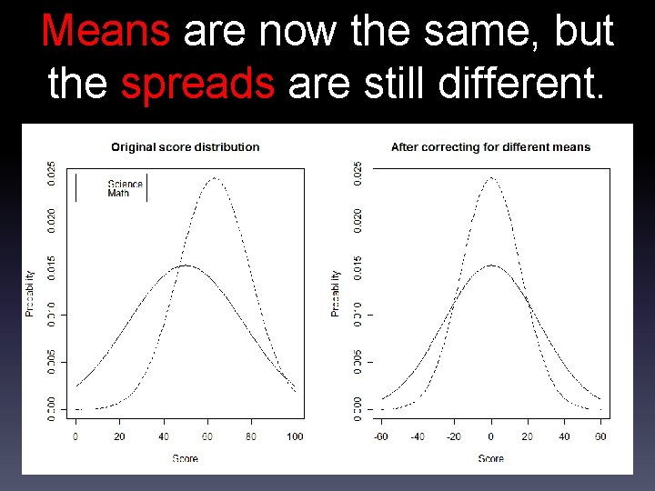
Means are now the same, but the spreads are still different. We still have a problem…Is a -35 on science the same as a -35 on math?

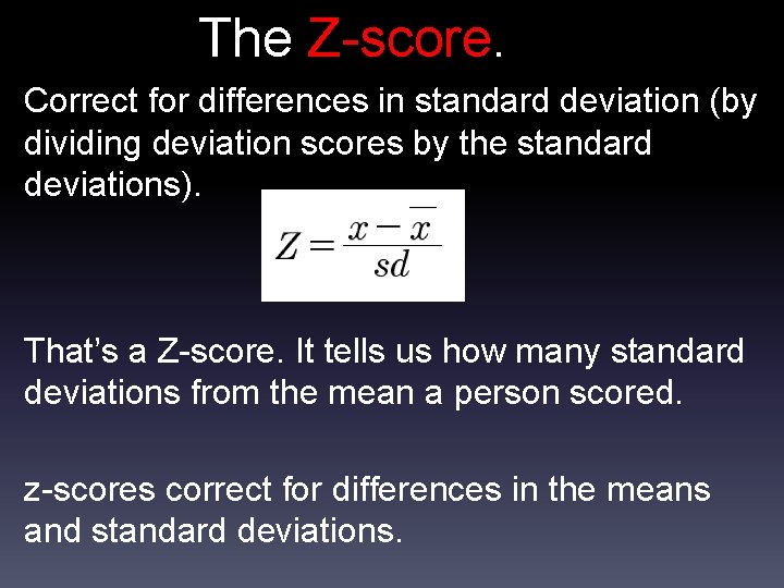
The Z-score. Correct for differences in standard deviation (by dividing deviation scores by the standard deviations). That’s a Z-score. It tells us how many standard deviations from the mean a person scored. z-scores correct for differences in the means and standard deviations.

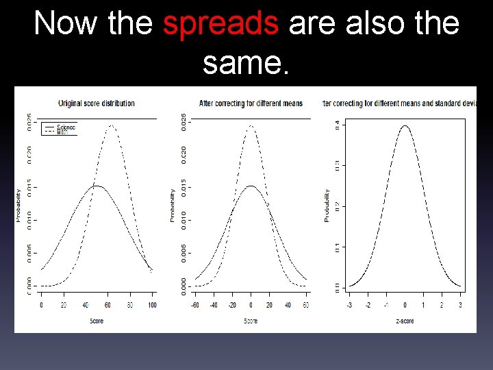
Now the spreads are also the same.

Areas under the normal curve. . 34 (34%) . 14 (14%) . 02 (2%). 0013 (. 13%) . 14 (14%) <-----68%-----> <-------95%-------> . 02 (2%) <-----------99%-----------> -3 sd -2 sd -1 sd Mean +1 sd +2 sd . 0013 (. 13%) +3 sd

Areas under the normal curve. . 34 (34%) . 14 (14%) . 02 (2%). 0013 (. 13%) . 14 (14%) <-----68%-----> <-------95%-------> . 02 (2%) <-----------99%-----------> -3 sd -2 sd -1 sd Mean +1 sd +2 sd . 0013 (. 13%) +3 sd

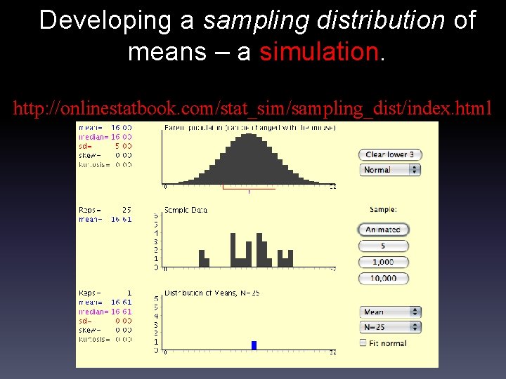
Developing a sampling distribution of means – a simulation. http: //onlinestatbook. com/stat_sim/sampling_dist/index. html

The Central Limit Theorem. The sampling distribution of means: Approaches an increasingly normal distribution as number of samples increases, regardless of the shape of the population from which the samples were drawn. Has a mean (i. e. , “mean of means”) that approaches to the population mean (“mu”) as the number of samples increases.

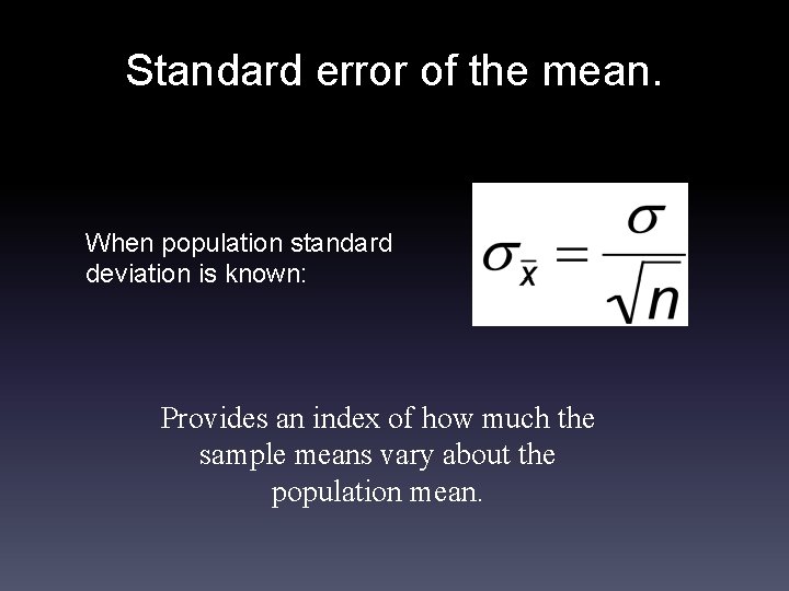
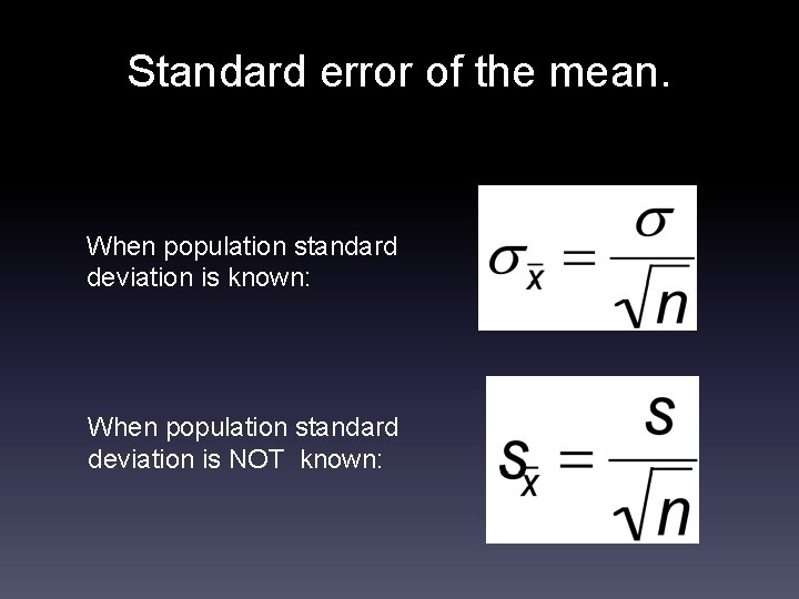
Standard error of the mean. When population standard deviation is known: Provides an index of how much the sample means vary about the population mean.

The recipe for constructing confidence intervals about the sample mean. Compute the standard error of the mean. Make a decision about level of confidence that is desired (usually 95% or 99%). Form 95% confidence interval by adding and subtracting 2 standard errors to and from the sample mean (+/- 3 standard errors for 99% confidence interval).

Hypothesis testing: case of a single sample. Does a particular sample of observations in this study come from a specified population or does it represent a different population? If the population standard deviation is known, use a Z-test to answer the question. If the population standard deviation is NOT known, use a ttest to answer the question.

Suppose you are the superintendent of schools and you are informed that the average reading achievement of your 4 th graders has fallen below that of the national average. One explanation posed by the teachers is that the district is faced with an unusually dull group of 4 th graders this year. The teachers suggest that the average verbal IQ of this year’s 4 th graders is below the national average, and that is why reading achievement is so low. You know that IQ-test scores don’t change much from year to year unless a school system is affected by systematic changes in its enrollment (e. g. , a large migration of new families). Your school system has remained quite stable in the past with a mean verbal IQ score of 100 and a standard deviation of 15 – both right at the national average. You have a limited budget, and while you have extensive achievement data on the 4 th graders, you have limited verbal IQ data available. So you decide to test a sample of 400 4 th graders rather than all 5000 of them. The verbal IQ mean for the sample is 102.

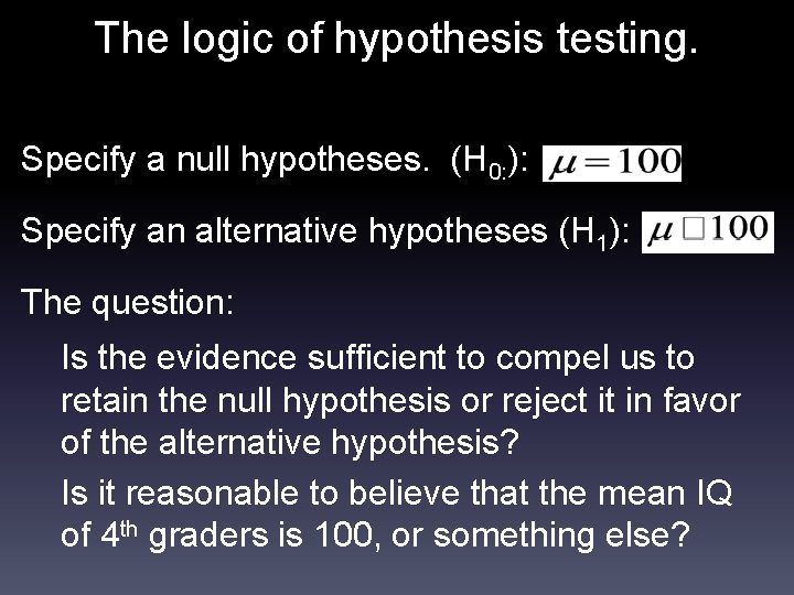
The logic of hypothesis testing. Specify a null hypotheses. (H 0: ): Specify an alternative hypotheses (H 1): The question: Is the evidence sufficient to compel us to retain the null hypothesis or reject it in favor of the alternative hypothesis? Is it reasonable to believe that the mean IQ of 4 th graders is 100, or something else?

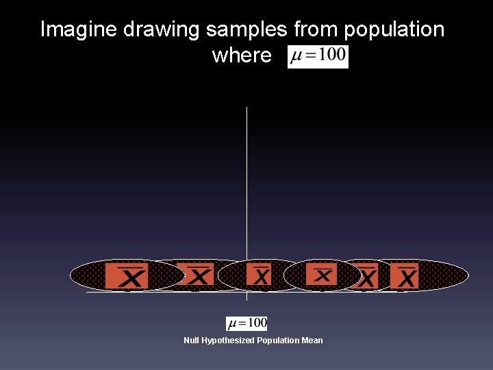
Imagine drawing samples from population where Null Hypothesized Population Mean

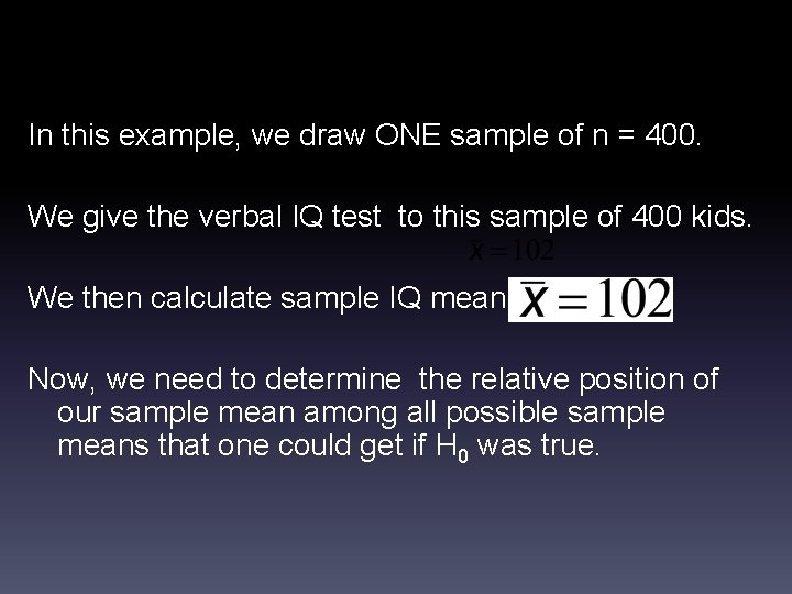
In this example, we draw ONE sample of n = 400. We give the verbal IQ test to this sample of 400 kids. We then calculate sample IQ mean: Now, we need to determine the relative position of our sample mean among all possible sample means that one could get if H 0 was true.

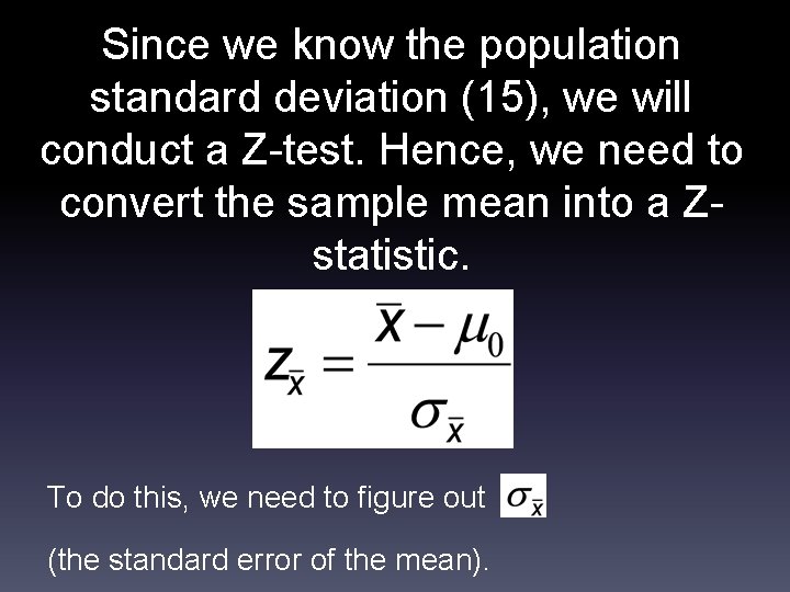
Since we know the population standard deviation (15), we will conduct a Z-test. Hence, we need to convert the sample mean into a Zstatistic. To do this, we need to figure out (the standard error of the mean).

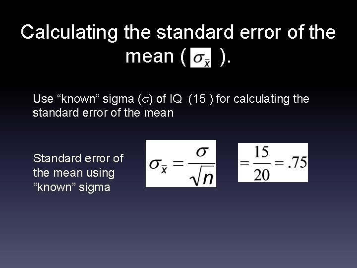
Calculating the standard error of the mean ( ). Use “known” sigma ( ) of IQ (15 ) for calculating the standard error of the mean Standard error of the mean using “known” sigma

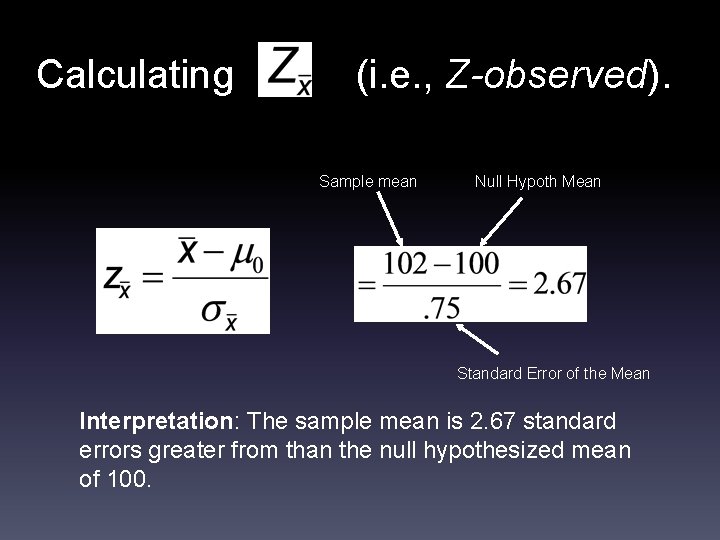
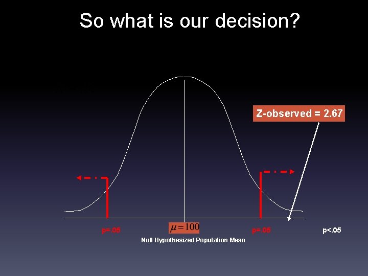
Calculating (i. e. , Z-observed). Sample mean Null Hypoth Mean Standard Error of the Mean Interpretation: The sample mean is 2. 67 standard errors greater from than the null hypothesized mean of 100.

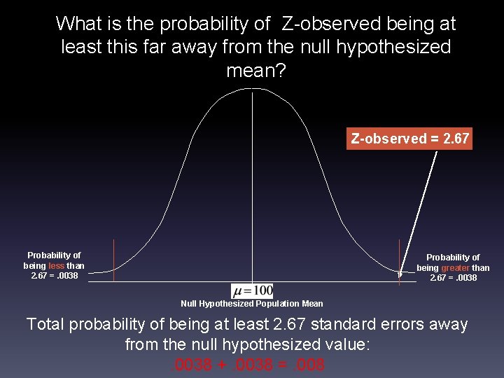
What is the probability of Z-observed being at least this far away from the null hypothesized mean? Z-observed = 2. 67 Probability of being less than 2. 67 =. 0038 Probability of being greater than 2. 67 =. 0038 Null Hypothesized Population Mean Total probability of being at least 2. 67 standard errors away from the null hypothesized value: . 0038 +. 0038 =. 008

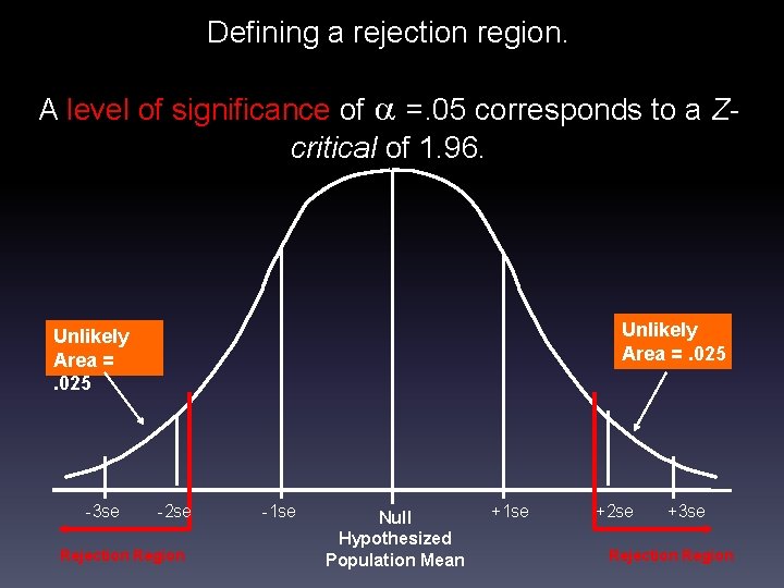
Defining a rejection region. A level of significance of =. 05 corresponds to a Zcritical of 1. 96. Unlikely Area =. 025 -3 se -2 se Rejection Region -1 se Null Hypothesized Population Mean +1 se +2 se +3 se Rejection Region

Time to make a decision. The level of significance ( ) sets your rejection region. Decision: Reject the null hypothesis H 0 at the significance level if the sample statistic falls in the rejection region. I. e. , the probability (p) of obtaining a sample statistic at least as large as observed is or less (p ≤ ). Fail to reject the null hypothesis H 0 at the significance level if the sample statistic falls outside the rejection region. I. e. , the probability (p) of obtaining a sample statistic at least as large as observed is more than (p > ).

So what is our decision? Z-observed = 2. 67 p=. 05 Null Hypothesized Population Mean p<. 05

Decision and conclusion. Decision: reject Ho, because the probability of getting a mean at least as large as 102 if the null hypothesis is true, is equal to or less than. 05 Getting a sample mean this deviant from the null hypothesized mean is highly unlikely under the null hypothesis of Conclusion: The result is statistically significant at the 5% significance level. The mean is statistically significantly higher than 100.

Determining the level of significance (i. e. , risk of Type I error). Usually select some small (conservative) level of significance. α =. 05: generally accepted level for social science. α =. 01, . 001: more conservative. The level of significance (� ) is a statement of risk. More specifically, it is a statement of the risk of falsely rejecting the null hypothesis that a researcher is willing to permit. This is known as Type I error.

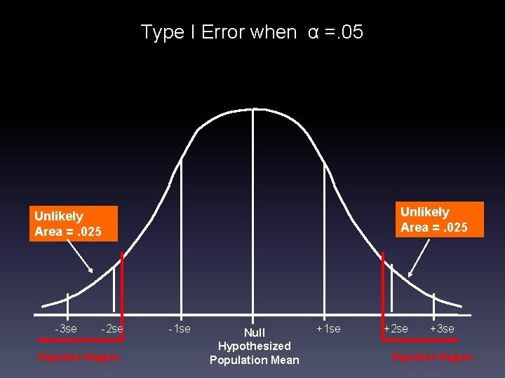
Type I Error when α =. 05 Unlikely Area =. 025 -3 se -2 se Rejection Region -1 se Null Hypothesized Population Mean +1 se +2 se +3 se Rejection Region

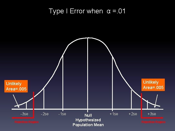
Type I Error when α =. 01 Unlikely Area=. 005 -3 se Rejection Region -2 se -1 se Null Hypothesized Population Mean +1 se +2 se +3 se Rejection Region

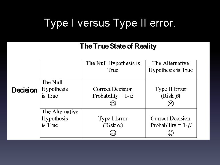
Type I versus Type II error.

Type II error (β). Type II Error: If the alternative hypothesis (HA) is true and the decision maker decides to stick with the null hypothesis (H 0). Reduce Type II error (β) by increasing sample size.

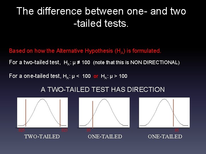
The difference between one- and two -tailed tests. Based on how the Alternative Hypothesis (HA) is formulated. For a two-tailed test, HA: μ ≠ 100 (note that this is NON DIRECTIONAL) For a one-tailed test, HA: μ < 100 or HA: μ > 100 A TWO-TAILED TEST HAS DIRECTION . 025 TWO-TAILED . 025 . 05 ONE-TAILED

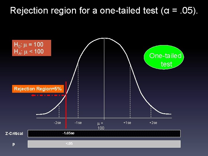
Rejection region for a one-tailed test (α =. 05). H 0: = 100 HA: < 100 One-tailed test Rejection Region=5% -2 se -1 se Z-Critical -1. 65 se p <. 05 = 100 +1 se +2 se

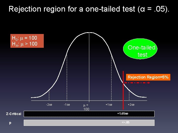
Rejection region for a one-tailed test (α =. 05). H 0: = 100 HA: > 100 One-tailed test Rejection Region=5% -2 se Z-Critical p -1 se = 100 +1 se +2 se +1. 65 se <=. 05

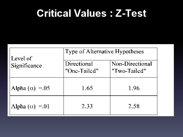
Critical Values : Z-Test

Standard error of the mean. When population standard deviation is known: When population standard deviation is NOT known:

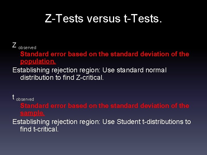
Z-Tests versus t-Tests. Z observed Standard error based on the standard deviation of the population. Establishing rejection region: Use standard normal distribution to find Z-critical. t observed Standard error based on the standard deviation of the sample. Establishing rejection region: Use Student t-distributions to find t-critical.

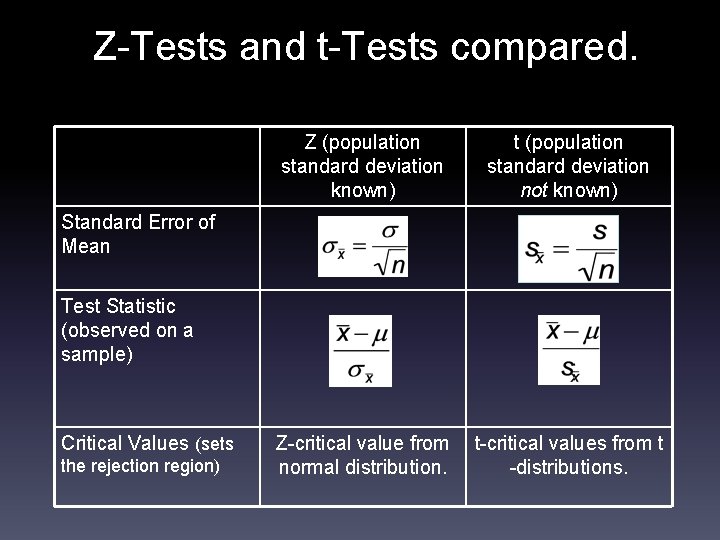
Z-Tests and t-Tests compared. Z (population standard deviation known) t (population standard deviation not known) Z-critical value from normal distribution. t-critical values from t -distributions. Standard Error of Mean Test Statistic (observed on a sample) Critical Values (sets the rejection region)

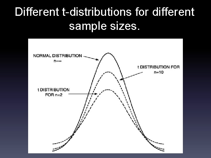
Different t-distributions for different sample sizes.

A unique t-distribution for every sample size. t-distributions differ according to their degrees of freedom, which are based on sample size (n). For a single sample the t-distribution is based on n-1 degrees of freedom (df). As n ∞, the t-distribution more and more closely resembles the normal distribution.

Two-sample t-tests. Is there a statistically significant difference between the means of two groups on a given variable of interest? In other words, do the two sets represent samples from identical or different populations?

Paired versus independent samples. Paired samples t-test. Compares two means based on related data. E. g. , data from the same people measured at different times, or data from “matched” samples. Independent samples t-test. Compares two means based on independent data. E. g. , data from different groups of people.

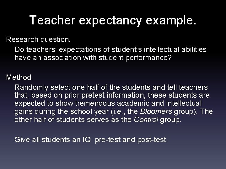
Teacher expectancy example. Research question. Do teachers’ expectations of student’s intellectual abilities have an association with student performance? Method. Randomly select one half of the students and tell teachers that, based on prior pretest information, these students are expected to show tremendous academic and intellectual gains during the school year (i. e. , the Bloomers group). The other half of students serves as the Control group. Give all students an IQ pre-test and post-test.

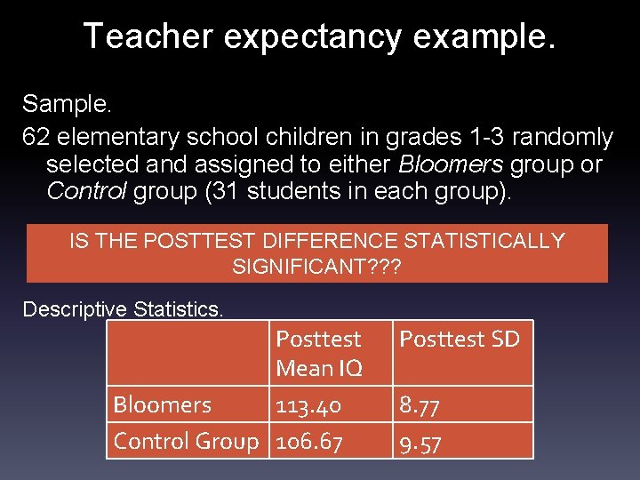
Teacher expectancy example. Sample. 62 elementary school children in grades 1 -3 randomly selected and assigned to either Bloomers group or Control group (31 students in each group). IS THE POSTTEST DIFFERENCE STATISTICALLY SIGNIFICANT? ? ? Descriptive Statistics. Posttest Mean IQ Bloomers 113. 40 Control Group 106. 67 Posttest SD 8. 77 9. 57

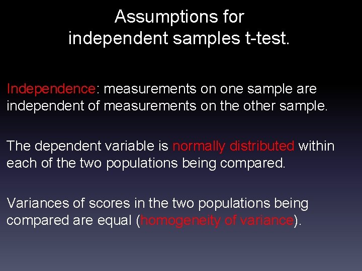
Assumptions for independent samples t-test. Independence: measurements on one sample are independent of measurements on the other sample. The dependent variable is normally distributed within each of the two populations being compared. Variances of scores in the two populations being compared are equal (homogeneity of variance).

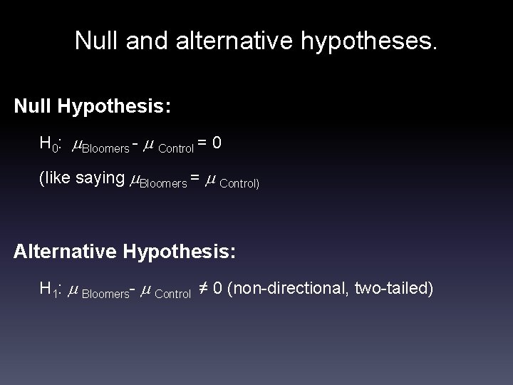
Null and alternative hypotheses. Null Hypothesis: H 0: Bloomers - Control = 0 (like saying Bloomers = Control) Alternative Hypothesis: H 1: Bloomers- Control ≠ 0 (non-directional, two-tailed)

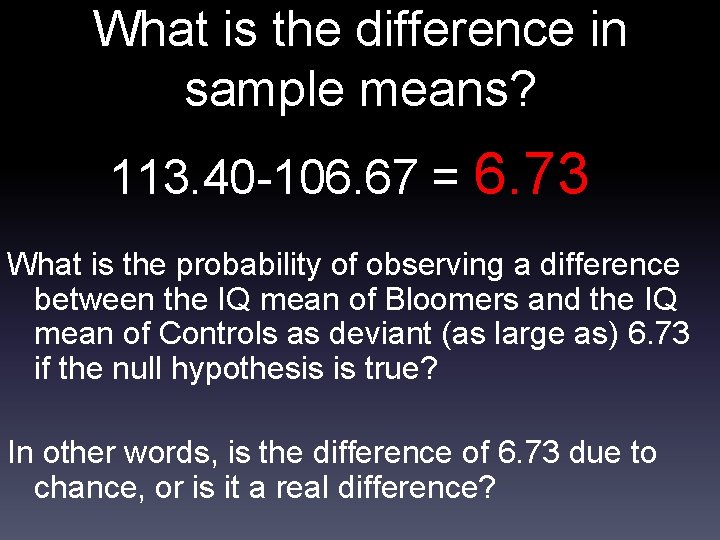
What is the difference in sample means? 113. 40 -106. 67 = 6. 73 What is the probability of observing a difference between the IQ mean of Bloomers and the IQ mean of Controls as deviant (as large as) 6. 73 if the null hypothesis is true? In other words, is the difference of 6. 73 due to chance, or is it a real difference?

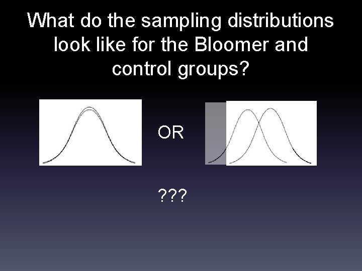
What do the sampling distributions look like for the Bloomer and control groups? OR ? ? ?

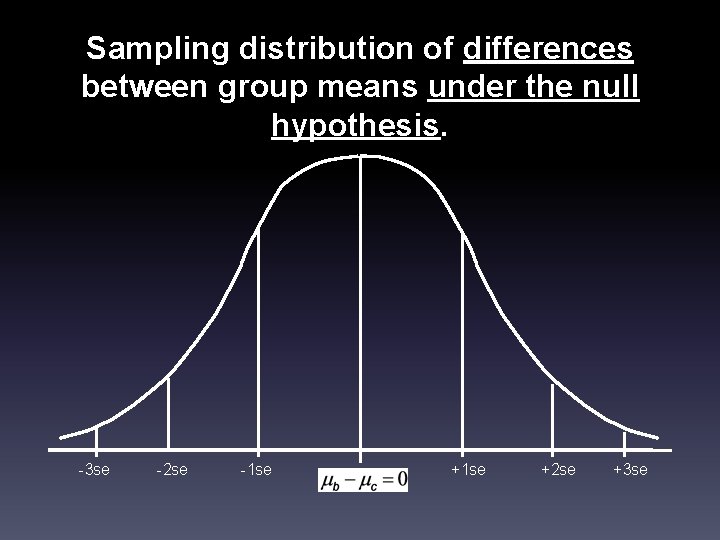
Sampling distribution of differences between group means under the null hypothesis. -3 se -2 se -1 se 0 +1 se +2 se +3 se

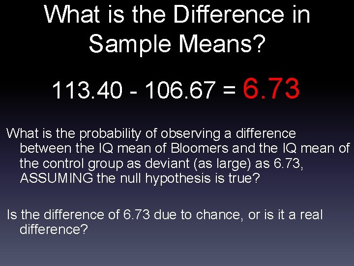
What is the Difference in Sample Means? 113. 40 - 106. 67 = 6. 73 What is the probability of observing a difference between the IQ mean of Bloomers and the IQ mean of the control group as deviant (as large) as 6. 73, ASSUMING the null hypothesis is true? Is the difference of 6. 73 due to chance, or is it a real difference?

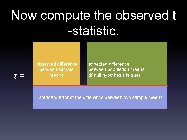
Now compute the observed t -statistic. t= observed difference between sample means − expected difference between population means (if null hypothesis is true) standard error of the difference between two sample means

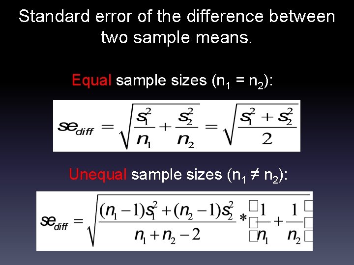
Standard error of the difference between two sample means. Equal sample sizes (n 1 = n 2): Unequal sample sizes (n 1 ≠ n 2):

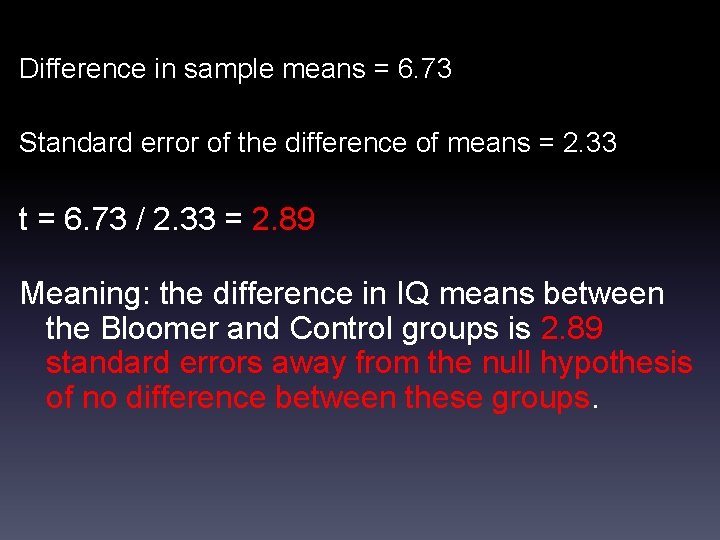
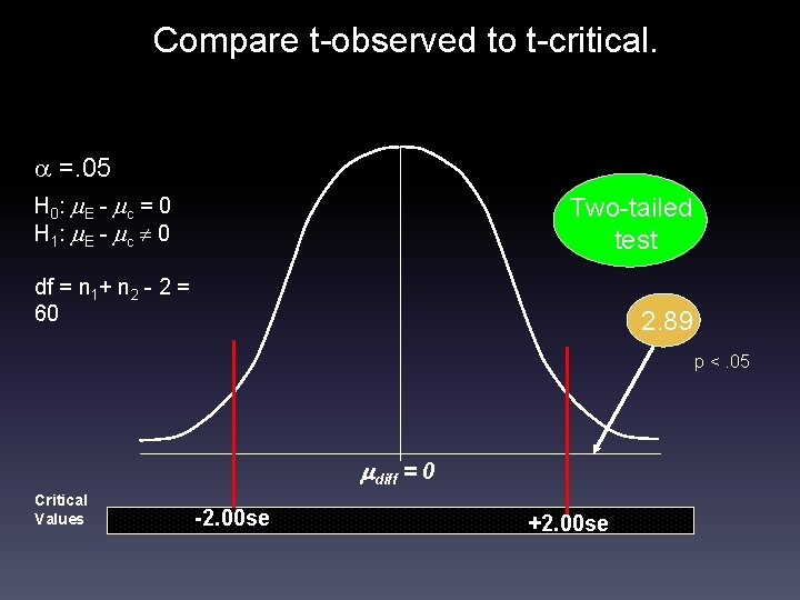
Difference in sample means = 6. 73 Standard error of the difference of means = 2. 33 t = 6. 73 / 2. 33 = 2. 89 Meaning: the difference in IQ means between the Bloomer and Control groups is 2. 89 standard errors away from the null hypothesis of no difference between these groups.

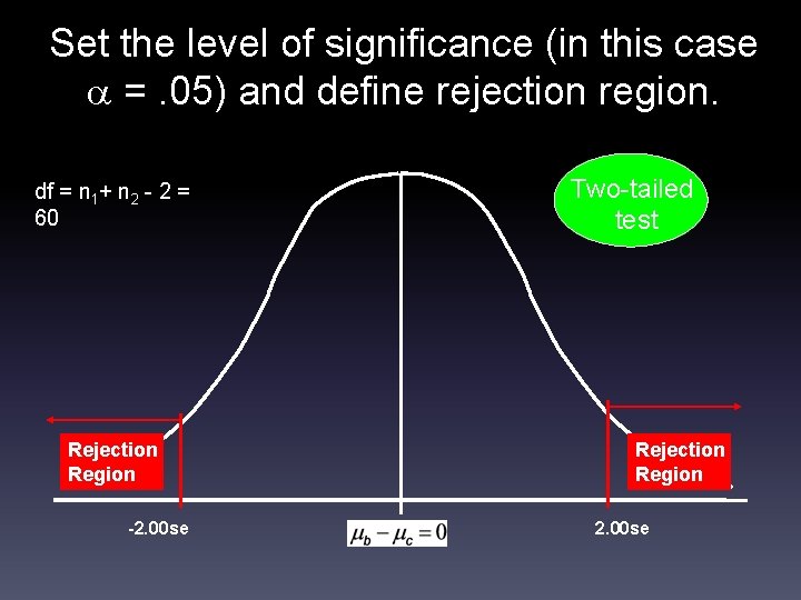
Set the level of significance (in this case =. 05) and define rejection region. df = n 1+ n 2 - 2 = 60 Rejection Region -2. 00 se Two-tailed test Rejection Region 2. 00 se

Compare t-observed to t-critical. =. 05 H 0 : E - c = 0 H 1 : E - c 0 Two-tailed test df = n 1+ n 2 - 2 = 60 2. 89 p <. 05 diff = 0 Critical Values -2. 00 se +2. 00 se

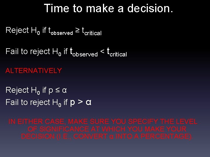
Time to make a decision. Reject H 0 if tobserved ≥ tcritical Fail to reject H 0 if tobserved < tcritical ALTERNATIVELY Reject H 0 if p ≤ α Fail to reject H 0 if p > α IN EITHER CASE, MAKE SURE YOU SPECIFY THE LEVEL OF SIGNIFICANCE AT WHICH YOU MAKE YOUR DECISION (I. E. , CONVERT α INTO A PERCENTAGE).

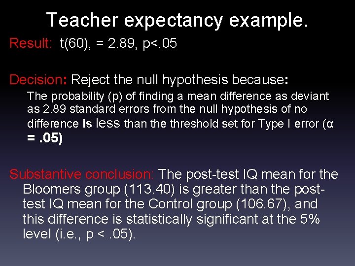
Teacher expectancy example. Result: t(60), = 2. 89, p<. 05 Decision: Reject the null hypothesis because: The probability (p) of finding a mean difference as deviant as 2. 89 standard errors from the null hypothesis of no difference is less than the threshold set for Type I error (α =. 05) Substantive conclusion: The post-test IQ mean for the Bloomers group (113. 40) is greater than the posttest IQ mean for the Control group (106. 67), and this difference is statistically significant at the 5% level (i. e. , p <. 05).

Practical significance. Statistically significant findings may not be practically significant. A common way of assessing practical significance: EFFECT SIZE.

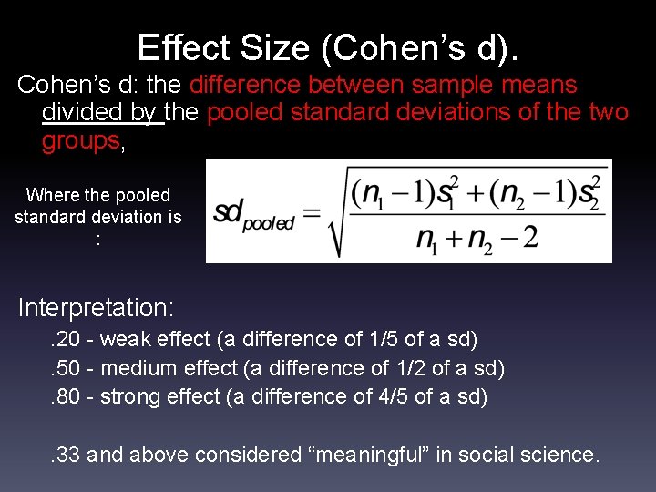
Effect Size (Cohen’s d). Cohen’s d: the difference between sample means divided by the pooled standard deviations of the two groups, Where the pooled standard deviation is : Interpretation: . 20 - weak effect (a difference of 1/5 of a sd). 50 - medium effect (a difference of 1/2 of a sd). 80 - strong effect (a difference of 4/5 of a sd). 33 and above considered “meaningful” in social science.

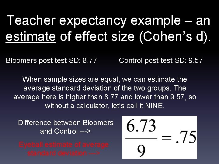
Teacher expectancy example – an estimate of effect size (Cohen’s d). Bloomers post-test SD: 8. 77 Control post-test SD: 9. 57 When sample sizes are equal, we can estimate the average standard deviation of the two groups. The average here is higher than 8. 77 and lower than 9. 57, so without a calculator, let’s call it NINE. Difference between Bloomers and Control ---> Eyeball estimate of average standard deviation --->