Edges Edge Detection Contour Segmentation Hough Transform Edges

Edges ØEdge Detection ØContour Segmentation ØHough Transform Edges Based on A Practical Introduction to Computer Vision with Open. CV by Kenneth Dawson-Howe © Wiley & Sons Inc. 2014 Slide 1

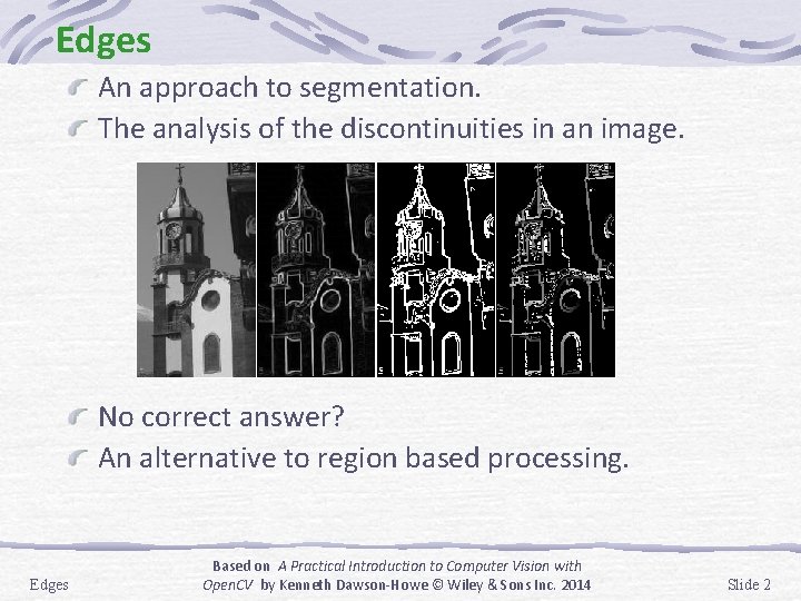
Edges An approach to segmentation. The analysis of the discontinuities in an image. No correct answer? An alternative to region based processing. Edges Based on A Practical Introduction to Computer Vision with Open. CV by Kenneth Dawson-Howe © Wiley & Sons Inc. 2014 Slide 2

Edge Detection – Topics 1 st derivative edge detection 2 nd derivative edge detection Multispectral edge detection Image sharpening Edges Based on A Practical Introduction to Computer Vision with Open. CV by Kenneth Dawson-Howe © Wiley & Sons Inc. 2014 Slide 3

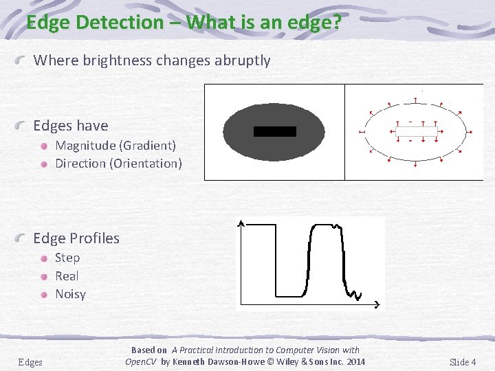
Edge Detection – What is an edge? Where brightness changes abruptly Edges have Magnitude (Gradient) Direction (Orientation) Edge Profiles Step Real Noisy Edges Based on A Practical Introduction to Computer Vision with Open. CV by Kenneth Dawson-Howe © Wiley & Sons Inc. 2014 Slide 4

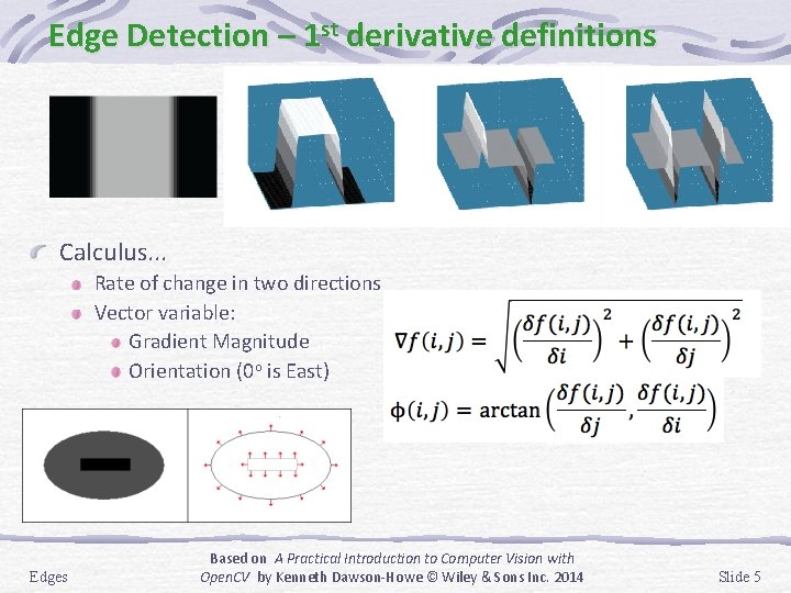
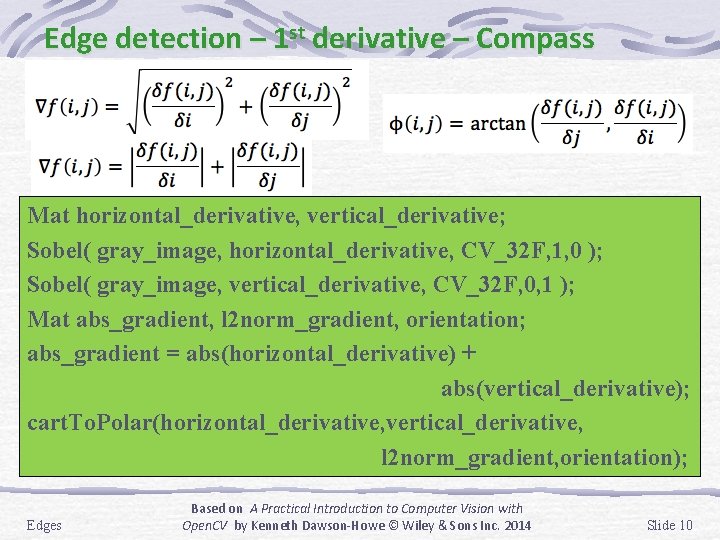
Edge Detection – 1 st derivative definitions Calculus. . . Rate of change in two directions Vector variable: Gradient Magnitude Orientation (0 o is East) Edges Based on A Practical Introduction to Computer Vision with Open. CV by Kenneth Dawson-Howe © Wiley & Sons Inc. 2014 Slide 5

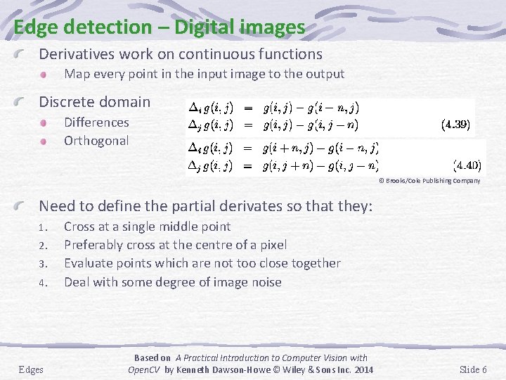
Edge detection – Digital images Derivatives work on continuous functions Map every point in the input image to the output Discrete domain Differences Orthogonal © Brooks/Cole Publishing Company Need to define the partial derivates so that they: 1. 2. 3. 4. Edges Cross at a single middle point Preferably cross at the centre of a pixel Evaluate points which are not too close together Deal with some degree of image noise Based on A Practical Introduction to Computer Vision with Open. CV by Kenneth Dawson-Howe © Wiley & Sons Inc. 2014 Slide 6

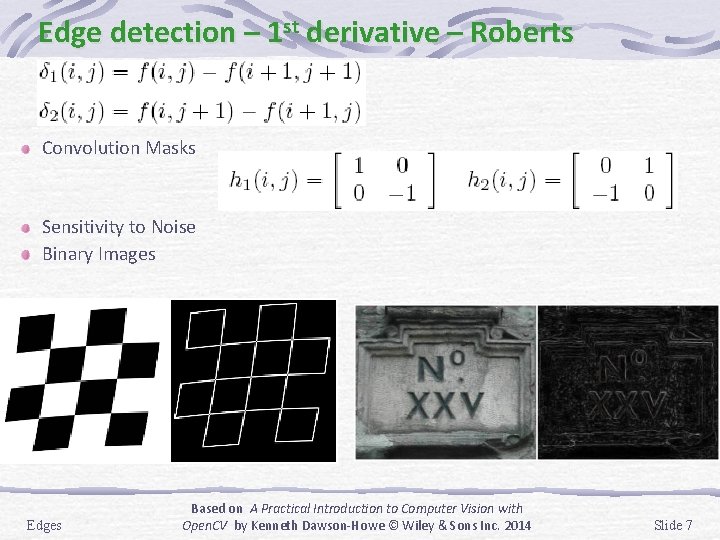
Edge detection – 1 st derivative – Roberts Convolution Masks Sensitivity to Noise Binary Images Edges Based on A Practical Introduction to Computer Vision with Open. CV by Kenneth Dawson-Howe © Wiley & Sons Inc. 2014 Slide 7

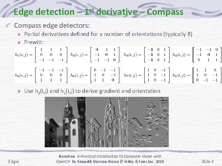
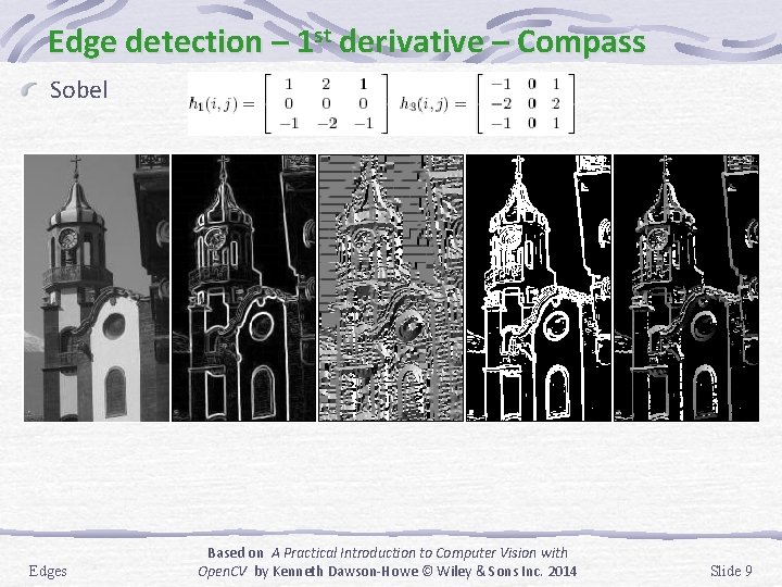
Edge detection – 1 st derivative – Compass edge detectors: Partial derivatives defined for a number of orientations (typically 8) Prewitt: Use h 3(i, j) and h 1(i, j) to derive gradient and orientation Edges Based on A Practical Introduction to Computer Vision with Open. CV by Kenneth Dawson-Howe © Wiley & Sons Inc. 2014 Slide 8

Edge detection – 1 st derivative – Compass Sobel Edges Based on A Practical Introduction to Computer Vision with Open. CV by Kenneth Dawson-Howe © Wiley & Sons Inc. 2014 Slide 9

Edge detection – 1 st derivative – Compass Mat horizontal_derivative, vertical_derivative; Sobel( gray_image, horizontal_derivative, CV_32 F, 1, 0 ); Sobel( gray_image, vertical_derivative, CV_32 F, 0, 1 ); Mat abs_gradient, l 2 norm_gradient, orientation; abs_gradient = abs(horizontal_derivative) + abs(vertical_derivative); cart. To. Polar(horizontal_derivative, vertical_derivative, l 2 norm_gradient, orientation); Edges Based on A Practical Introduction to Computer Vision with Open. CV by Kenneth Dawson-Howe © Wiley & Sons Inc. 2014 Slide 10

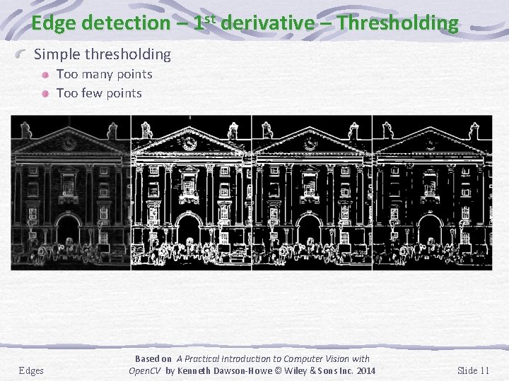
Edge detection – 1 st derivative – Thresholding Simple thresholding Too many points Too few points Edges Based on A Practical Introduction to Computer Vision with Open. CV by Kenneth Dawson-Howe © Wiley & Sons Inc. 2014 Slide 11

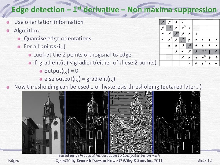
Edge detection – 1 st derivative – Non maxima suppression Use orientation information Algorithm: Quantise edge orientations For all points (i, j) Look at the 2 points orthogonal to edge if gradient(i, j) < gradient(either of these 2 points) output(i, j) = 0 else output(i, j) = gradient(i, j) Now thresholding can be used… or hysteresis thresholding (detailed later…) Edges Based on A Practical Introduction to Computer Vision with Open. CV by Kenneth Dawson-Howe © Wiley & Sons Inc. 2014 Slide 12

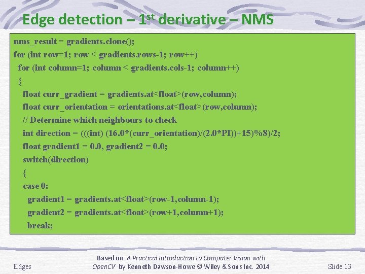
Edge detection – 1 st derivative – NMS nms_result = gradients. clone(); for (int row=1; row < gradients. rows-1; row++) for (int column=1; column < gradients. cols-1; column++) { float curr_gradient = gradients. at<float>(row, column); float curr_orientation = orientations. at<float>(row, column); // Determine which neighbours to check int direction = (((int) (16. 0*(curr_orientation)/(2. 0*PI))+15)%8)/2; float gradient 1 = 0. 0, gradient 2 = 0. 0; switch(direction) { case 0: gradient 1 = gradients. at<float>(row-1, column-1); gradient 2 = gradients. at<float>(row+1, column+1); break; Edges Based on A Practical Introduction to Computer Vision with Open. CV by Kenneth Dawson-Howe © Wiley & Sons Inc. 2014 Slide 13

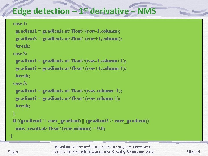
Edge detection – 1 st derivative – NMS case 1: gradient 1 = gradients. at<float>(row-1, column); gradient 2 = gradients. at<float>(row+1, column); break; case 2: gradient 1 = gradients. at<float>(row-1, column+1); gradient 2 = gradients. at<float>(row+1, column-1); break; case 3: gradient 1 = gradients. at<float>(row, column+1); gradient 2 = gradients. at<float>(row, column-1); break; } if ((gradient 1 > curr_gradient) || (gradient 2 > curr_gradient)) nms_result. at<float>(row, column) = 0. 0; } Edges Based on A Practical Introduction to Computer Vision with Open. CV by Kenneth Dawson-Howe © Wiley & Sons Inc. 2014 Slide 14

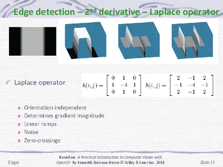
Edge detection – 2 nd derivative – Laplace operator Orientation independent Determines gradient magnitude Linear ramps Noise Zero-crossings Edges Based on A Practical Introduction to Computer Vision with Open. CV by Kenneth Dawson-Howe © Wiley & Sons Inc. 2014 Slide 15

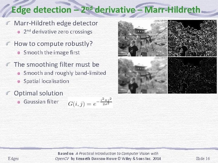
Edge detection – 2 nd derivative – Marr-Hildreth edge detector 2 nd derivative zero crossings How to compute robustly? Smooth the image first The smoothing filter must be Smooth and roughly band-limited Spatial localisation Optimal solution Gaussian filter Edges Based on A Practical Introduction to Computer Vision with Open. CV by Kenneth Dawson-Howe © Wiley & Sons Inc. 2014 Slide 16

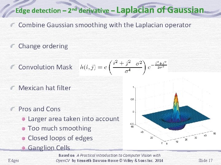
Edge detection – 2 nd derivative – Laplacian of Gaussian Combine Gaussian smoothing with the Laplacian operator Change ordering Convolution Mask Mexican hat filter Pros and Cons Larger area taken into account Too much smoothing Closed loops of edges Ganglion Cells Edges Based on A Practical Introduction to Computer Vision with Open. CV by Kenneth Dawson-Howe © Wiley & Sons Inc. 2014 Slide 17

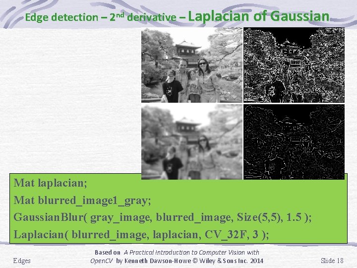
Edge detection – 2 nd derivative – Laplacian of Gaussian Mat laplacian; Mat blurred_image 1_gray; Gaussian. Blur( gray_image, blurred_image, Size(5, 5), 1. 5 ); Laplacian( blurred_image, laplacian, CV_32 F, 3 ); Edges Based on A Practical Introduction to Computer Vision with Open. CV by Kenneth Dawson-Howe © Wiley & Sons Inc. 2014 Slide 18

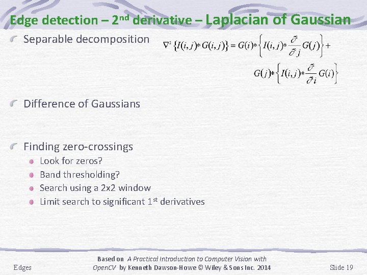
Edge detection – 2 nd derivative – Laplacian of Gaussian Separable decomposition Difference of Gaussians Finding zero-crossings Look for zeros? Band thresholding? Search using a 2 x 2 window Limit search to significant 1 st derivatives Edges Based on A Practical Introduction to Computer Vision with Open. CV by Kenneth Dawson-Howe © Wiley & Sons Inc. 2014 Slide 19

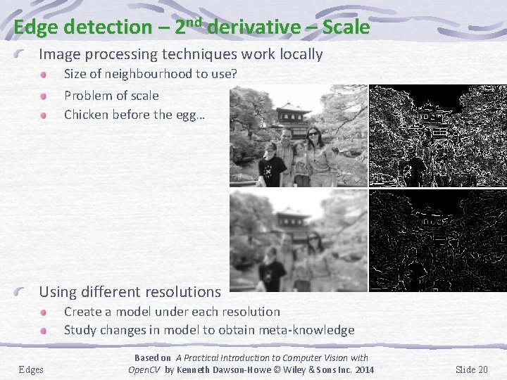
Edge detection – 2 nd derivative – Scale Image processing techniques work locally Size of neighbourhood to use? Problem of scale Chicken before the egg… Using different resolutions Create a model under each resolution Study changes in model to obtain meta-knowledge Edges Based on A Practical Introduction to Computer Vision with Open. CV by Kenneth Dawson-Howe © Wiley & Sons Inc. 2014 Slide 20

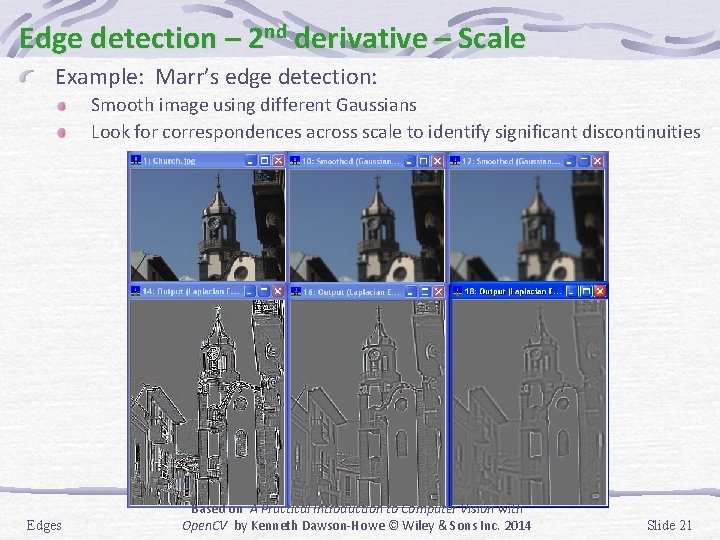
Edge detection – 2 nd derivative – Scale Example: Marr’s edge detection: Smooth image using different Gaussians Look for correspondences across scale to identify significant discontinuities Edges Based on A Practical Introduction to Computer Vision with Open. CV by Kenneth Dawson-Howe © Wiley & Sons Inc. 2014 Slide 21

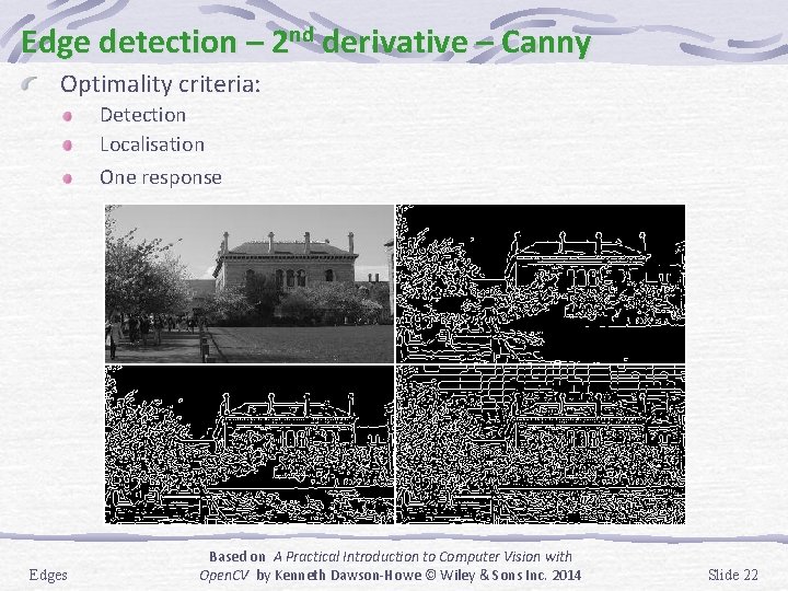
Edge detection – 2 nd derivative – Canny Optimality criteria: Detection Localisation One response Edges Based on A Practical Introduction to Computer Vision with Open. CV by Kenneth Dawson-Howe © Wiley & Sons Inc. 2014 Slide 22

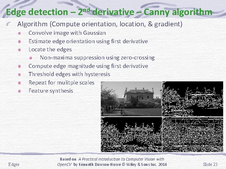
Edge detection – 2 nd derivative – Canny algorithm Algorithm (Compute orientation, location, & gradient) Convolve image with Gaussian Estimate edge orientation using first derivative Locate the edges Non-maxima suppression using zero-crossing Compute edge magnitude using first derivative Threshold edges with hysteresis Repeat for mulitple scales Feature synthesis Edges Based on A Practical Introduction to Computer Vision with Open. CV by Kenneth Dawson-Howe © Wiley & Sons Inc. 2014 Slide 23

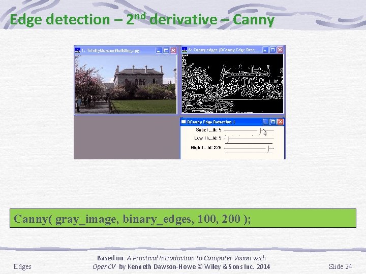
Edge detection – 2 nd derivative – Canny( gray_image, binary_edges, 100, 200 ); Edges Based on A Practical Introduction to Computer Vision with Open. CV by Kenneth Dawson-Howe © Wiley & Sons Inc. 2014 Slide 24

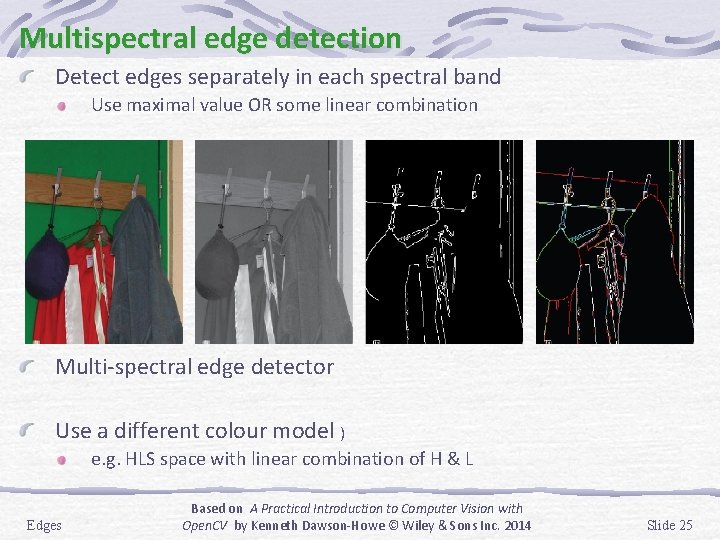
Multispectral edge detection Detect edges separately in each spectral band Use maximal value OR some linear combination Multi-spectral edge detector Use a different colour model ) e. g. HLS space with linear combination of H & L Edges Based on A Practical Introduction to Computer Vision with Open. CV by Kenneth Dawson-Howe © Wiley & Sons Inc. 2014 Slide 25

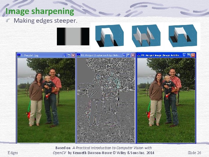
Image sharpening Making edges steeper. Demo (Sharpening. twk) Edges Based on A Practical Introduction to Computer Vision with Open. CV by Kenneth Dawson-Howe © Wiley & Sons Inc. 2014 Slide 26

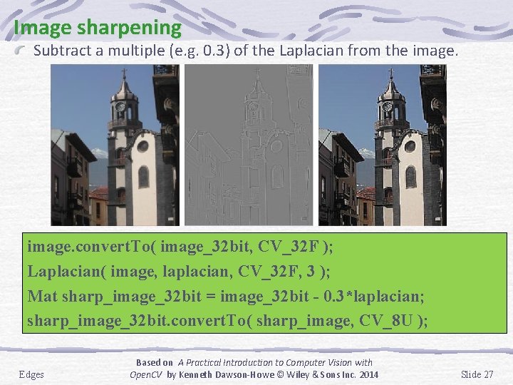
Image sharpening Subtract a multiple (e. g. 0. 3) of the Laplacian from the image. convert. To( image_32 bit, CV_32 F ); Laplacian( image, laplacian, CV_32 F, 3 ); Mat sharp_image_32 bit = image_32 bit - 0. 3*laplacian; sharp_image_32 bit. convert. To( sharp_image, CV_8 U ); Edges Based on A Practical Introduction to Computer Vision with Open. CV by Kenneth Dawson-Howe © Wiley & Sons Inc. 2014 Slide 27

Contour Segmentation – Topics Edge data representations Border Detection Line segment extraction Edges Based on A Practical Introduction to Computer Vision with Open. CV by Kenneth Dawson-Howe © Wiley & Sons Inc. 2014 Slide 28

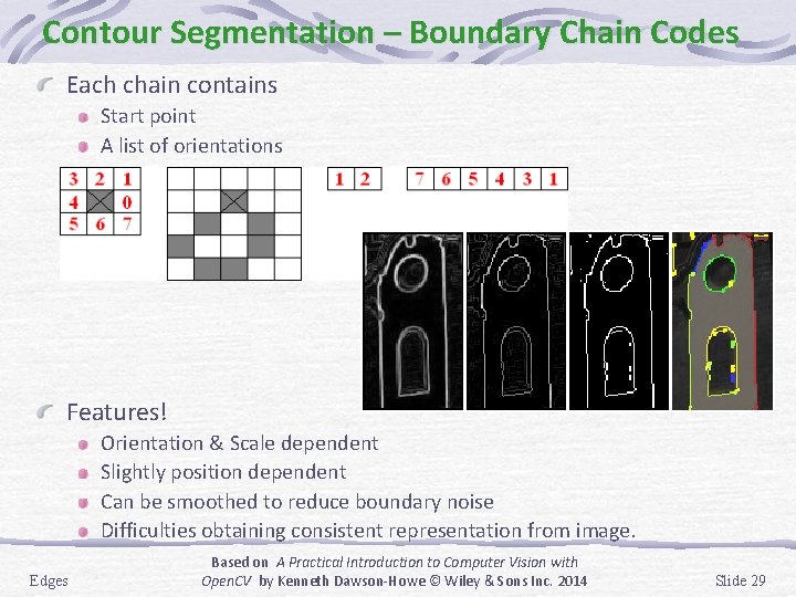
Contour Segmentation – Boundary Chain Codes Each chain contains Start point A list of orientations Features! Orientation & Scale dependent Slightly position dependent Can be smoothed to reduce boundary noise Difficulties obtaining consistent representation from image. Edges Based on A Practical Introduction to Computer Vision with Open. CV by Kenneth Dawson-Howe © Wiley & Sons Inc. 2014 Slide 29

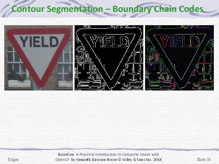
Contour Segmentation – Boundary Chain Codes Edges Based on A Practical Introduction to Computer Vision with Open. CV by Kenneth Dawson-Howe © Wiley & Sons Inc. 2014 Slide 30

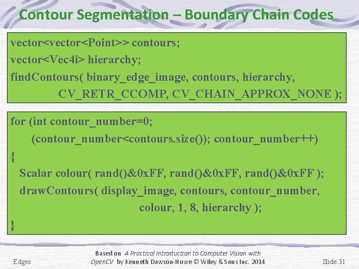
Contour Segmentation – Boundary Chain Codes vector<Point>> contours; vector<Vec 4 i> hierarchy; find. Contours( binary_edge_image, contours, hierarchy, CV_RETR_CCOMP, CV_CHAIN_APPROX_NONE ); for (int contour_number=0; (contour_number<contours. size()); contour_number++) { Scalar colour( rand()&0 x. FF, rand()&0 x. FF ); draw. Contours( display_image, contours, contour_number, colour, 1, 8, hierarchy ); } Edges Based on A Practical Introduction to Computer Vision with Open. CV by Kenneth Dawson-Howe © Wiley & Sons Inc. 2014 Slide 31

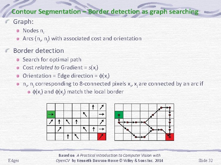
Contour Segmentation – Border detection as graph searching Graph: Nodes ni Arcs (ni, nj) with associated cost and orientation Border detection Search for optimal path Cost related to Gradient = s(xi) Orientation = Edge direction = (xi) ni, nj corresponding to 8 -connected pixels xi, xj are connected by an arc if (xi) and (xj) match the local border Edges Based on A Practical Introduction to Computer Vision with Open. CV by Kenneth Dawson-Howe © Wiley & Sons Inc. 2014 Slide 32

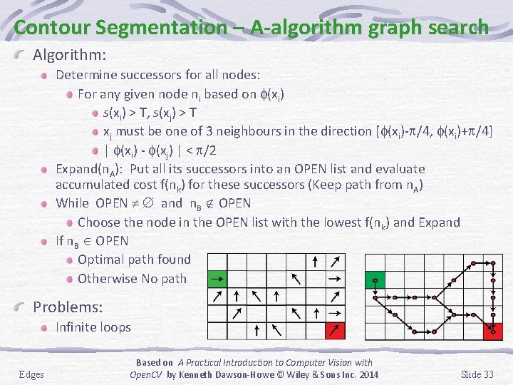
Contour Segmentation – A-algorithm graph search Algorithm: Determine successors for all nodes: For any given node ni based on (xi) s(xi) > T, s(xj) > T xj must be one of 3 neighbours in the direction [ (xi)- /4, (xi)+ /4] | (xi) - (xj) | < /2 Expand(n. A): Put all its successors into an OPEN list and evaluate accumulated cost f(nk) for these successors (Keep path from n. A) While OPEN and n. B OPEN Choose the node in the OPEN list with the lowest f(nk) and Expand If n. B OPEN Optimal path found Otherwise No path Problems: Infinite loops Edges Based on A Practical Introduction to Computer Vision with Open. CV by Kenneth Dawson-Howe © Wiley & Sons Inc. 2014 Slide 33

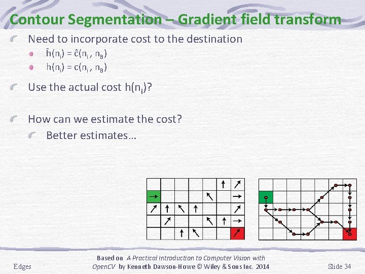
Contour Segmentation – Gradient field transform Need to incorporate cost to the destination ĥ(ni) = ĉ(ni , n. B) h(ni) = c(ni , n. B) Use the actual cost h(ni)? How can we estimate the cost? Better estimates… Edges Based on A Practical Introduction to Computer Vision with Open. CV by Kenneth Dawson-Howe © Wiley & Sons Inc. 2014 Slide 34

Contour Segmentation – Estimating the cost Cost so far Strength of edges (maximage s(xk)) - s(xi) Almost always gives good results Border curvature diff[ (xi) - (xj) ] Remaining cost… Proximity to an approximate border dist(xi, approximate_boundary) Distance to the goal dist(xi, x. B) Edges Based on A Practical Introduction to Computer Vision with Open. CV by Kenneth Dawson-Howe © Wiley & Sons Inc. 2014 Slide 35

Contour Segmentation – More efficient search Pruning the solution tree High average cost per unit length Maximum cost Max. path cost. Depth first search Reduce candidate edges Multi-resolution processing Determine approximate boundary first Incorporation of higher-level knowledge A priori knowledge Edges Based on A Practical Introduction to Computer Vision with Open. CV by Kenneth Dawson-Howe © Wiley & Sons Inc. 2014 Slide 36

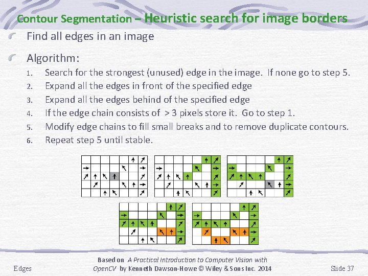
Contour Segmentation – Heuristic search for image borders Find all edges in an image Algorithm: 1. 2. 3. 4. 5. 6. Edges Search for the strongest (unused) edge in the image. If none go to step 5. Expand all the edges in front of the specified edge Expand all the edges behind of the specified edge If the edge chain consists of > 3 pixels store it. Go to step 1. Modify edge chains to fill small breaks and to remove duplicate contours. Repeat step 5 until stable. Based on A Practical Introduction to Computer Vision with Open. CV by Kenneth Dawson-Howe © Wiley & Sons Inc. 2014 Slide 37

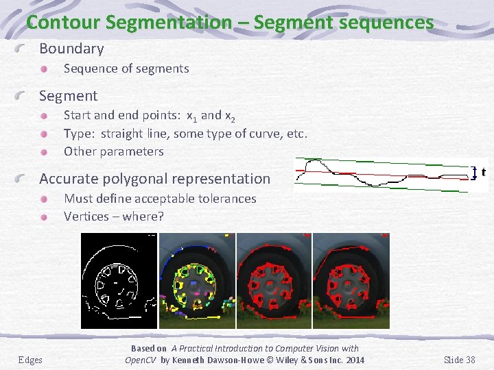
Contour Segmentation – Segment sequences Boundary Sequence of segments Segment Start and end points: x 1 and x 2 Type: straight line, some type of curve, etc. Other parameters Accurate polygonal representation Must define acceptable tolerances Vertices – where? Edges Based on A Practical Introduction to Computer Vision with Open. CV by Kenneth Dawson-Howe © Wiley & Sons Inc. 2014 Slide 38

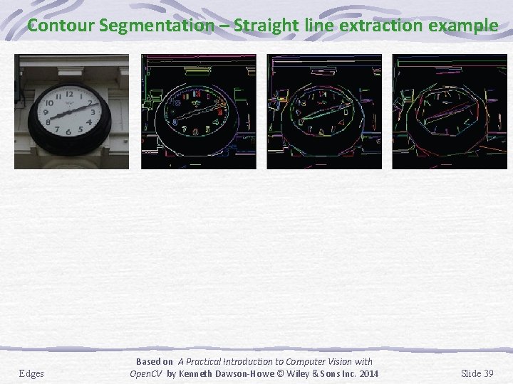
Contour Segmentation – Straight line extraction example Edges Based on A Practical Introduction to Computer Vision with Open. CV by Kenneth Dawson-Howe © Wiley & Sons Inc. 2014 Slide 39

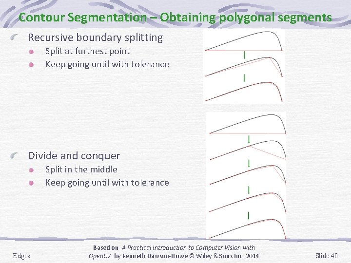
Contour Segmentation – Obtaining polygonal segments Recursive boundary splitting Split at furthest point Keep going until with tolerance Divide and conquer Split in the middle Keep going until with tolerance Edges Based on A Practical Introduction to Computer Vision with Open. CV by Kenneth Dawson-Howe © Wiley & Sons Inc. 2014 Slide 40

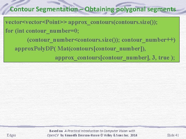
Contour Segmentation – Obtaining polygonal segments vector<Point>> approx_contours(contours. size()); for (int contour_number=0; (contour_number<contours. size()); contour_number++) approx. Poly. DP( Mat(contours[contour_number]), approx_contours[contour_number], 3, true ); Edges Based on A Practical Introduction to Computer Vision with Open. CV by Kenneth Dawson-Howe © Wiley & Sons Inc. 2014 Slide 41

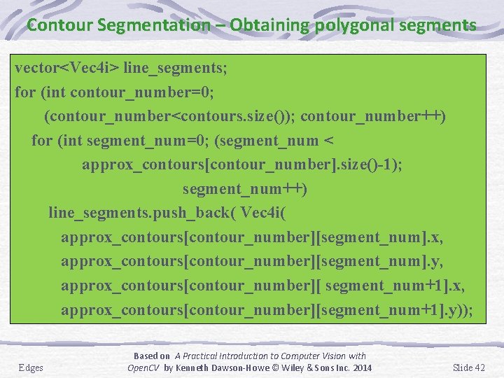
Contour Segmentation – Obtaining polygonal segments vector<Vec 4 i> line_segments; for (int contour_number=0; (contour_number<contours. size()); contour_number++) for (int segment_num=0; (segment_num < approx_contours[contour_number]. size()-1); segment_num++) line_segments. push_back( Vec 4 i( approx_contours[contour_number][segment_num]. x, approx_contours[contour_number][segment_num]. y, approx_contours[contour_number][ segment_num+1]. x, approx_contours[contour_number][segment_num+1]. y)); Edges Based on A Practical Introduction to Computer Vision with Open. CV by Kenneth Dawson-Howe © Wiley & Sons Inc. 2014 Slide 42

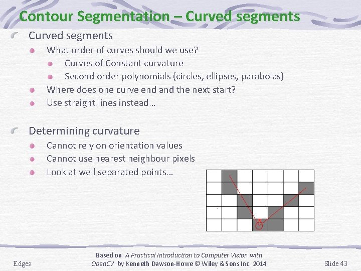
Contour Segmentation – Curved segments What order of curves should we use? Curves of Constant curvature Second order polynomials (circles, ellipses, parabolas) Where does one curve end and the next start? Use straight lines instead… Determining curvature Cannot rely on orientation values Cannot use nearest neighbour pixels Look at well separated points… Edges Based on A Practical Introduction to Computer Vision with Open. CV by Kenneth Dawson-Howe © Wiley & Sons Inc. 2014 Slide 43

Hough Transform – Topics Hough for lines Hough for circles Generalised Hough Edges Based on A Practical Introduction to Computer Vision with Open. CV by Kenneth Dawson-Howe © Wiley & Sons Inc. 2014 Slide 44

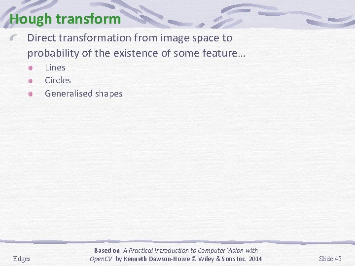
Hough transform Direct transformation from image space to probability of the existence of some feature… Lines Circles Generalised shapes Edges Based on A Practical Introduction to Computer Vision with Open. CV by Kenneth Dawson-Howe © Wiley & Sons Inc. 2014 Slide 45

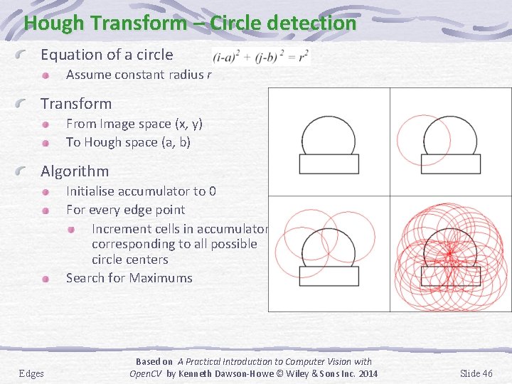
Hough Transform – Circle detection Equation of a circle Assume constant radius r Transform From Image space (x, y) To Hough space (a, b) Algorithm Initialise accumulator to 0 For every edge point Increment cells in accumulator corresponding to all possible circle centers Search for Maximums Edges Based on A Practical Introduction to Computer Vision with Open. CV by Kenneth Dawson-Howe © Wiley & Sons Inc. 2014 Slide 46

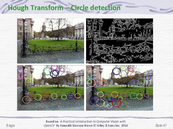
Hough Transform – Circle detection Edges Based on A Practical Introduction to Computer Vision with Open. CV by Kenneth Dawson-Howe © Wiley & Sons Inc. 2014 Slide 47

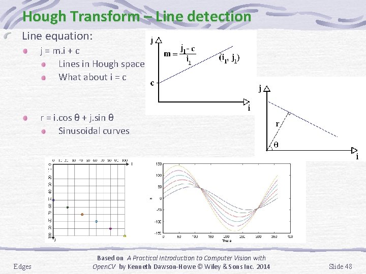
Hough Transform – Line detection Line equation: j = m. i + c Lines in Hough space What about i = c r = i. cos θ + j. sin θ Sinusoidal curves Edges Based on A Practical Introduction to Computer Vision with Open. CV by Kenneth Dawson-Howe © Wiley & Sons Inc. 2014 Slide 48

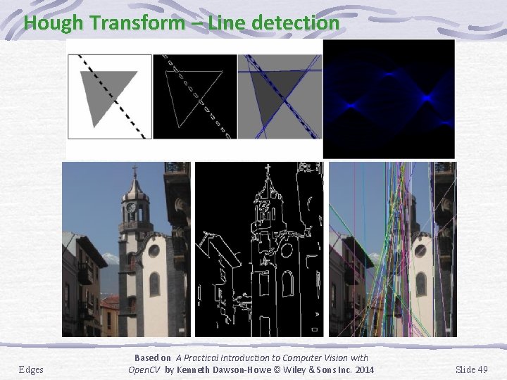
Hough Transform – Line detection Edges Based on A Practical Introduction to Computer Vision with Open. CV by Kenneth Dawson-Howe © Wiley & Sons Inc. 2014 Slide 49

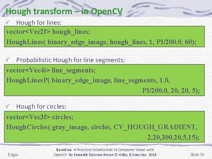
Hough transform – in Open. CV Hough for lines: vector<Vec 2 f> hough_lines; Hough. Lines( binary_edge_image, hough_lines, 1, PI/200. 0, 60); Probabilistic Hough for line segments: vector<Vec 4 i> line_segments; Hough. Lines. P( binary_edge_image, line_segments, 1. 0, PI/200. 0, 20, 5); Hough for circles: vector<Vec 3 f> circles; Hough. Circles( gray_image, circles, CV_HOUGH_GRADIENT, 2, 20, 300, 20, 5, 15); Edges Based on A Practical Introduction to Computer Vision with Open. CV by Kenneth Dawson-Howe © Wiley & Sons Inc. 2014 Slide 50

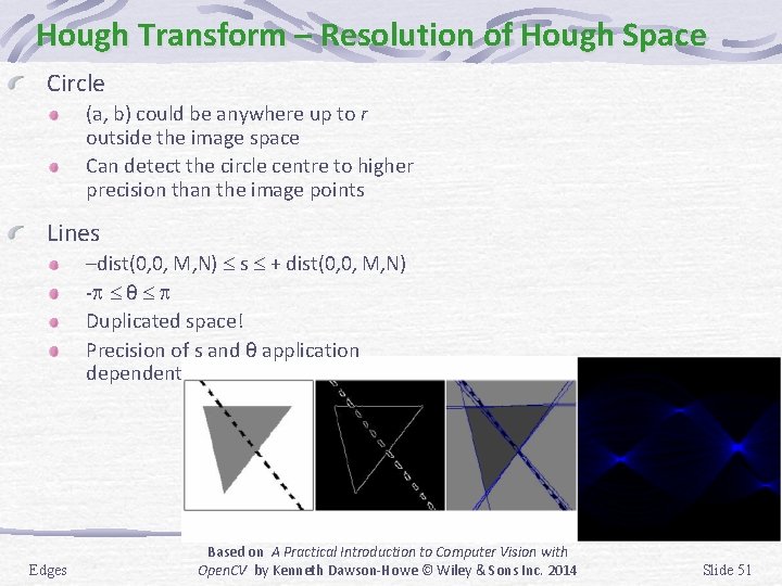
Hough Transform – Resolution of Hough Space Circle (a, b) could be anywhere up to r outside the image space Can detect the circle centre to higher precision than the image points Lines –dist(0, 0, M, N) s + dist(0, 0, M, N) - θ Duplicated space! Precision of s and θ application dependent Edges Based on A Practical Introduction to Computer Vision with Open. CV by Kenneth Dawson-Howe © Wiley & Sons Inc. 2014 Slide 51

Hough Transform – Efficient Implementation Use edge orientations Restrict the mapping into space Use half the accumulator For lines only Multi-resolution Process at a small resolution Higher resolution to find accurate data Problem What if the size of the circle is unknown 3 -D Accumulator? ? Edges Based on A Practical Introduction to Computer Vision with Open. CV by Kenneth Dawson-Howe © Wiley & Sons Inc. 2014 Slide 52

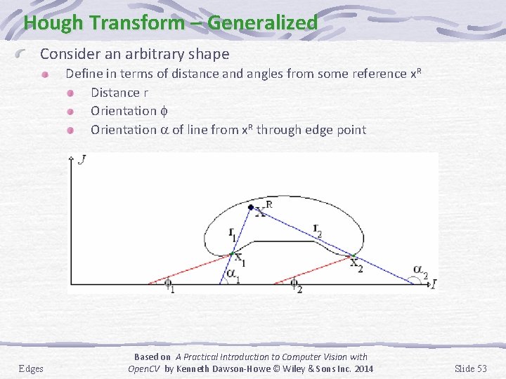
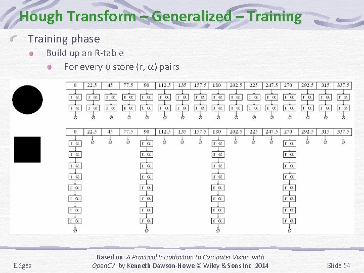
Hough Transform – Generalized Consider an arbitrary shape Define in terms of distance and angles from some reference x. R Distance r Orientation of line from x. R through edge point Edges Based on A Practical Introduction to Computer Vision with Open. CV by Kenneth Dawson-Howe © Wiley & Sons Inc. 2014 Slide 53

Hough Transform – Generalized – Training phase Build up an R-table For every store (r, ) pairs Edges Based on A Practical Introduction to Computer Vision with Open. CV by Kenneth Dawson-Howe © Wiley & Sons Inc. 2014 Slide 54

Hough Transform – Generalized – Recognition phase Create an accumulator for x. R For every edge point Determine its orientation Select a list of (r, ) pairs from the R-table Determine the position of x. R for each ( , r, ) and increment the accumulator appropriately Search for maximums Edges Based on A Practical Introduction to Computer Vision with Open. CV by Kenneth Dawson-Howe © Wiley & Sons Inc. 2014 Slide 55