EDGE DETECTION Instructor Dr Engr Junaid Zafar CONTENTS

EDGE DETECTION Instructor: Dr. Engr. Junaid Zafar

CONTENTS o o Introduction Types of Edges Steps in Edge Detection Methods of Edge Detection n o o o First Order Derivative Methods - Summary Second Order Derivative Methods o Second Order Derivative Methods - Summary Optimal Edge Detectors o Canny Edge Detection Edge Detector Performance Line Detection n Convolution based technique n Hough transform Application areas 2

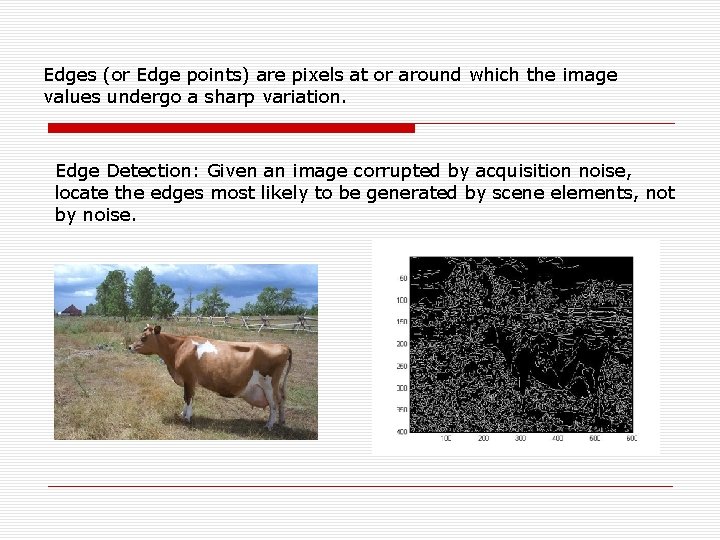
Edges (or Edge points) are pixels at or around which the image values undergo a sharp variation. Edge Detection: Given an image corrupted by acquisition noise, locate the edges most likely to be generated by scene elements, not by noise.

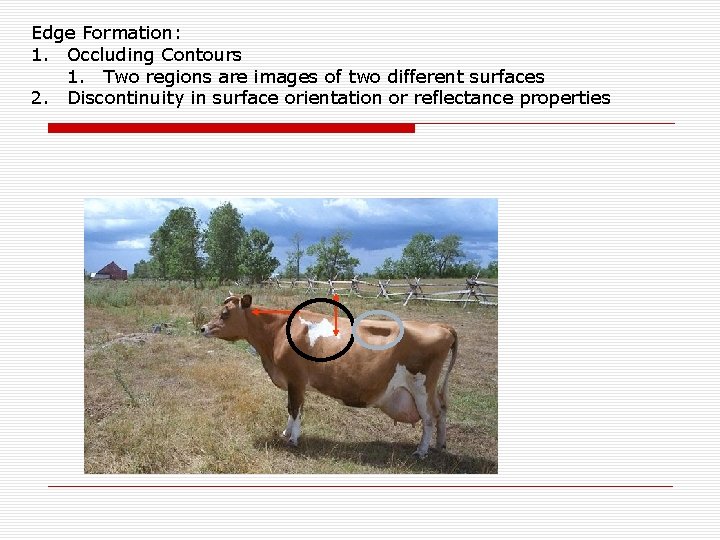
Edge Formation: 1. Occluding Contours 1. Two regions are images of two different surfaces 2. Discontinuity in surface orientation or reflectance properties

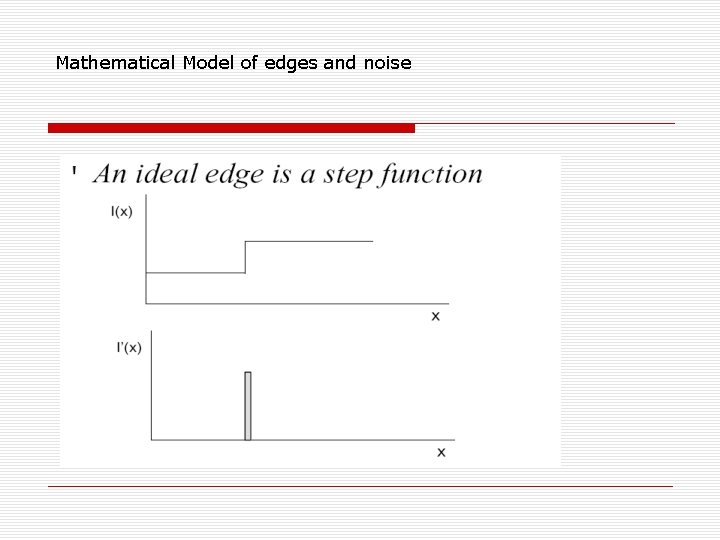
Mathematical Model of edges and noise

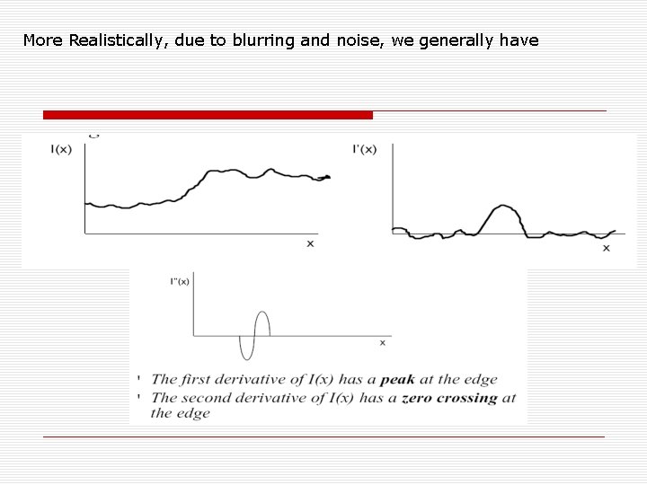
More Realistically, due to blurring and noise, we generally have

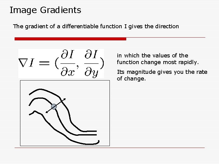
Image Gradients The gradient of a differentiable function I gives the direction in which the values of the function change most rapidly. Its magnitude gives you the rate of change.

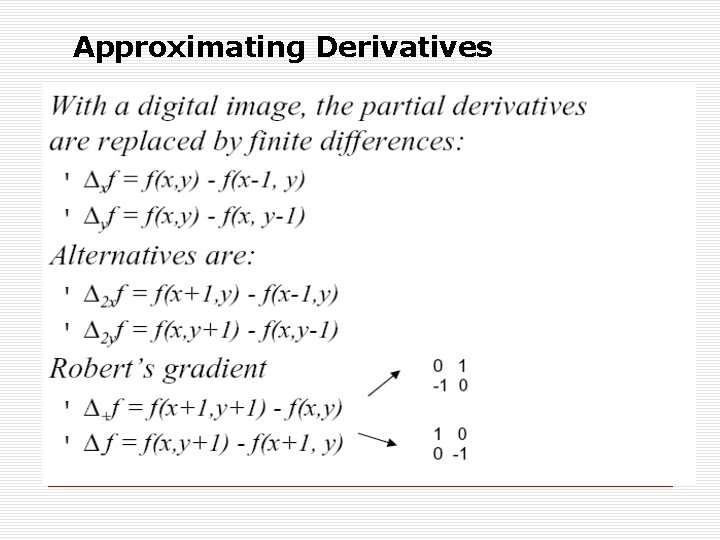
Approximating Derivatives

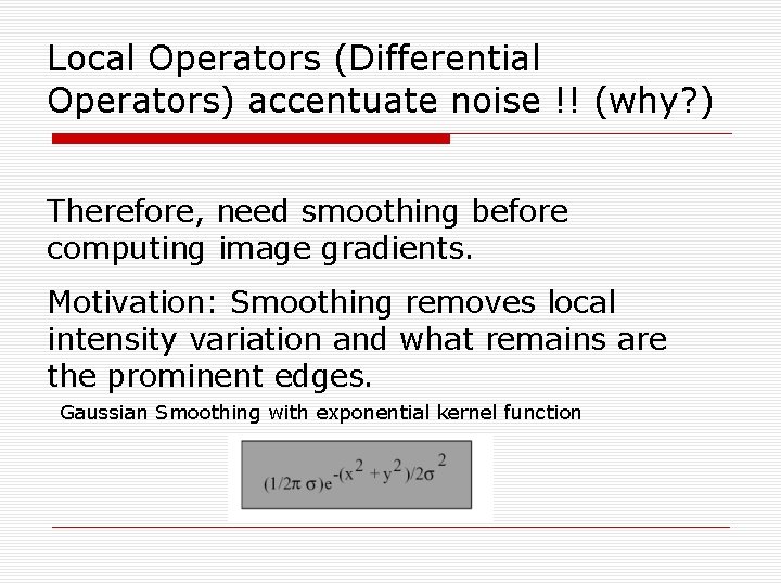
Local Operators (Differential Operators) accentuate noise !! (why? ) Therefore, need smoothing before computing image gradients. Motivation: Smoothing removes local intensity variation and what remains are the prominent edges. Gaussian Smoothing with exponential kernel function

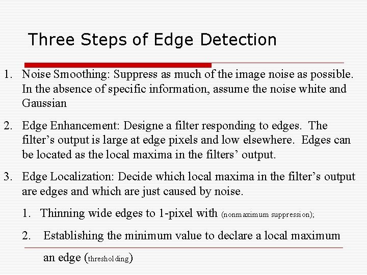
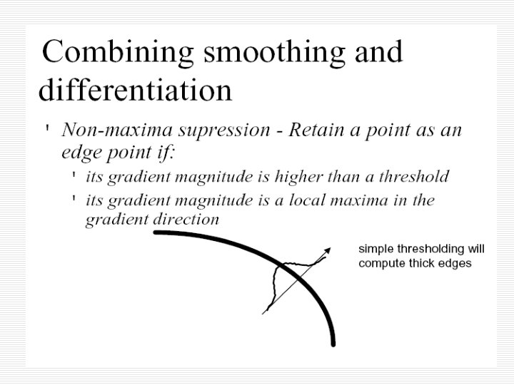
Three Steps of Edge Detection 1. Noise Smoothing: Suppress as much of the image noise as possible. In the absence of specific information, assume the noise white and Gaussian 2. Edge Enhancement: Designe a filter responding to edges. The filter’s output is large at edge pixels and low elsewhere. Edges can be located as the local maxima in the filters’ output. 3. Edge Localization: Decide which local maxima in the filter’s output are edges and which are just caused by noise. 1. Thinning wide edges to 1 -pixel with (nonmaximum suppression); 2. Establishing the minimum value to declare a local maximum an edge (thresholding)

Edge Descriptors (The output of an edge detector) 1. Edge normal: The direction of the maximum intensity variation at the edge point. 2. Edge direction: The direction tangent to the edge. 3. Edge Position : The location of the edge in image 4. Edge strength: A measure of local image contrast. How significance the intensity variation is across the edge.

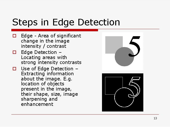
Steps in Edge Detection o Edge - Area of significant change in the image intensity / contrast o Edge Detection – Locating areas with strong intensity contrasts o Use of Edge Detection – Extracting information about the image. E. g. location of objects present in the image, their shape, size, image sharpening and enhancement 13

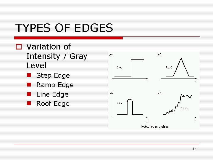
TYPES OF EDGES o Variation of Intensity / Gray Level n n Step Edge Ramp Edge Line Edge Roof Edge 14

Steps in Edge Detection o Filtering – Filter image to improve performance of the Edge Detector wrt noise o Enhancement – Emphasize pixels having significant change in local intensity o Detection – Identify edges - thresholding o Localization – Locate the edge accurately, estimate edge orientation 15

METHODS OF EDGE DETECTION o First Order Derivative / Gradient Methods n Roberts Operator n Sobel Operator n Prewitt Operator o Second Order Derivative n Laplacian of Gaussian n Difference of Gaussian o Optimal Edge Detection n Canny Edge Detection 16

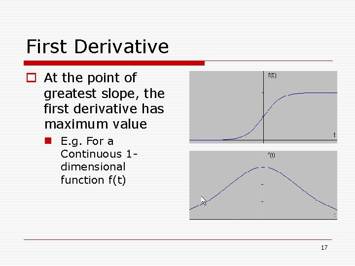
First Derivative o At the point of greatest slope, the first derivative has maximum value n E. g. For a Continuous 1 dimensional function f(t) 17

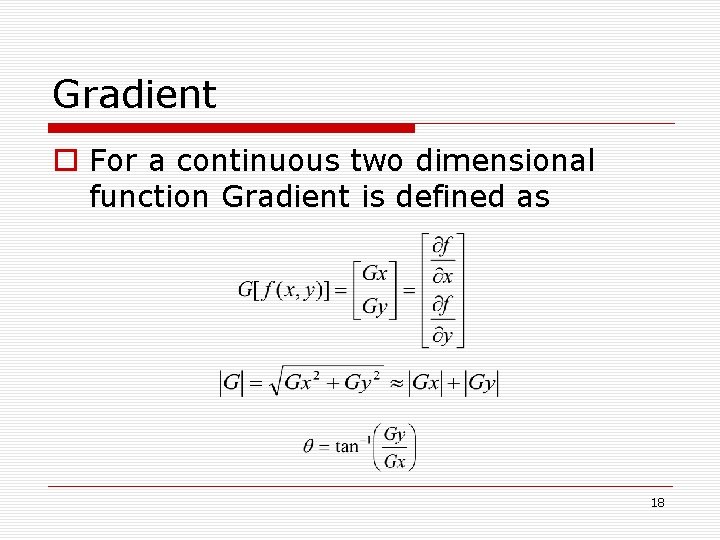
Gradient o For a continuous two dimensional function Gradient is defined as 18

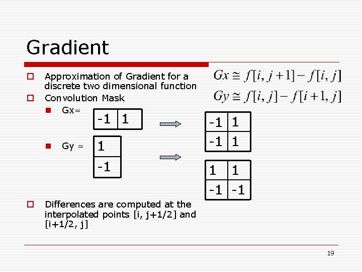
Gradient o o Approximation of Gradient for a discrete two dimensional function Convolution Mask n Gx= -1 1 n Gy = 1 -1 o -1 1 1 1 -1 -1 Differences are computed at the interpolated points [i, j+1/2] and [i+1/2, j] 19

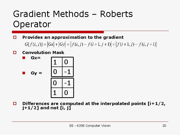
Gradient Methods – Roberts Operator o Provides an approximation to the gradient o Convolution Mask n Gx= n o Gy = 1 0 0 -1 0 1 -1 0 Differences are computed at the interpolated points [i+1/2, j+1/2] and not [i, j] EE - 6358 Computer Vision 20

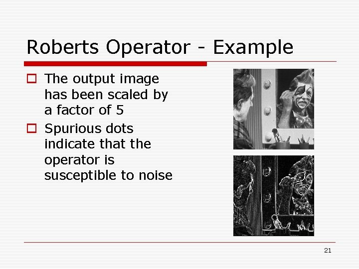
Roberts Operator - Example o The output image has been scaled by a factor of 5 o Spurious dots indicate that the operator is susceptible to noise 21

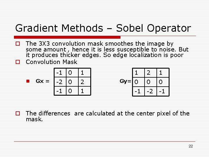
Gradient Methods – Sobel Operator o The 3 X 3 convolution mask smoothes the image by some amount , hence it is less susceptible to noise. But it produces thicker edges. So edge localization is poor o Convolution Mask n Gx = -1 0 1 1 2 1 -2 0 2 Gy= 0 0 0 -1 0 1 -2 -1 -1 o The differences are calculated at the center pixel of the mask. 22

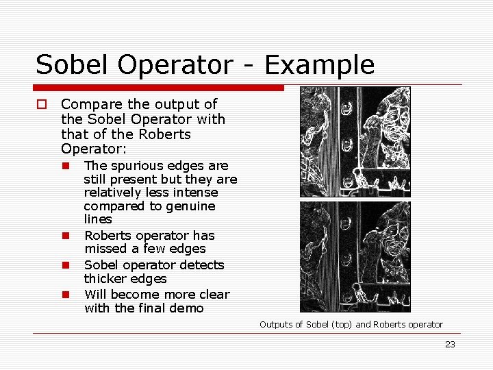
Sobel Operator - Example o Compare the output of the Sobel Operator with that of the Roberts Operator: n n The spurious edges are still present but they are relatively less intense compared to genuine lines Roberts operator has missed a few edges Sobel operator detects thicker edges Will become more clear with the final demo Outputs of Sobel (top) and Roberts operator 23

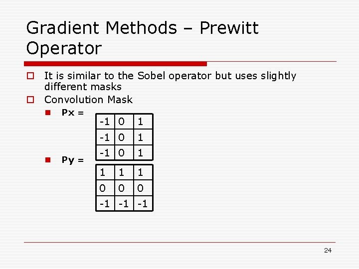
Gradient Methods – Prewitt Operator o It is similar to the Sobel operator but uses slightly different masks o Convolution Mask n n Px = Py = -1 0 1 1 0 0 0 -1 -1 -1 24

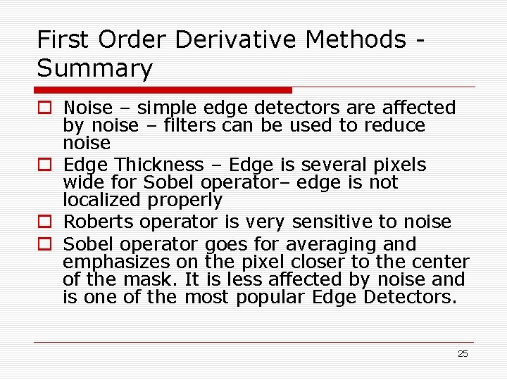
First Order Derivative Methods Summary o Noise – simple edge detectors are affected by noise – filters can be used to reduce noise o Edge Thickness – Edge is several pixels wide for Sobel operator– edge is not localized properly o Roberts operator is very sensitive to noise o Sobel operator goes for averaging and emphasizes on the pixel closer to the center of the mask. It is less affected by noise and is one of the most popular Edge Detectors. 25

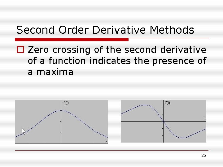
Second Order Derivative Methods o Zero crossing of the second derivative of a function indicates the presence of a maxima 26

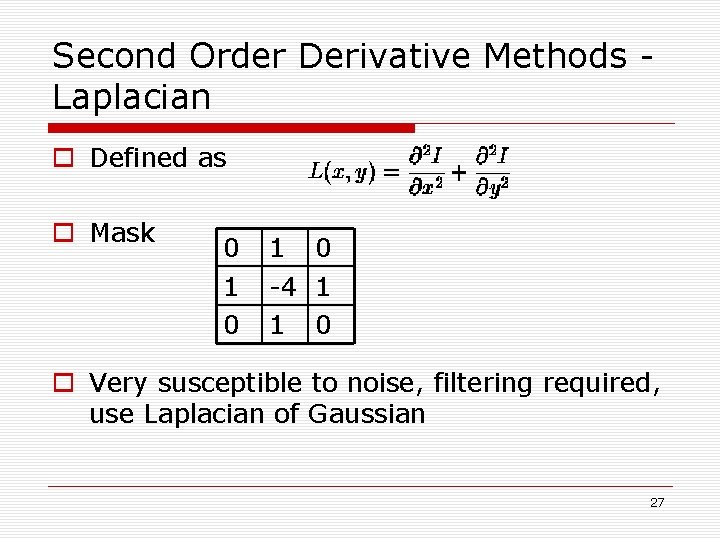
Second Order Derivative Methods Laplacian o Defined as o Mask 0 1 0 -4 1 1 0 o Very susceptible to noise, filtering required, use Laplacian of Gaussian 27

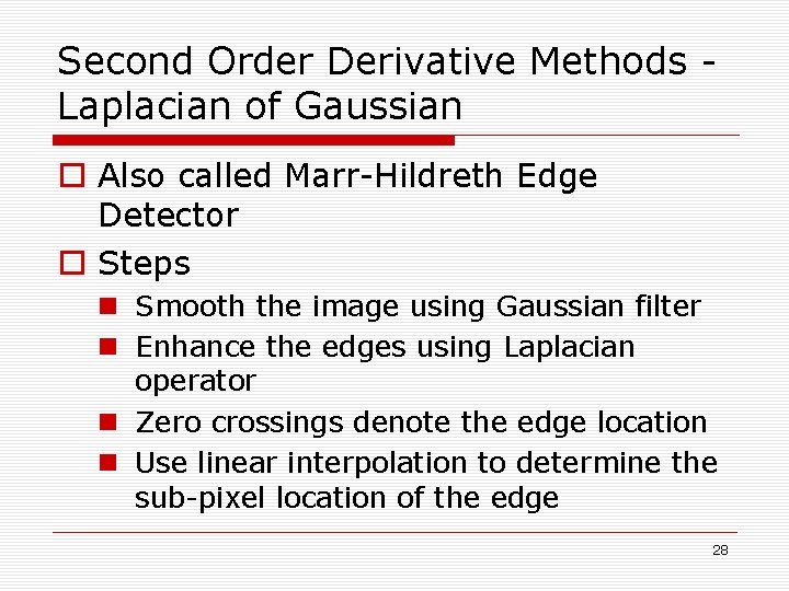
Second Order Derivative Methods Laplacian of Gaussian o Also called Marr-Hildreth Edge Detector o Steps n Smooth the image using Gaussian filter n Enhance the edges using Laplacian operator n Zero crossings denote the edge location n Use linear interpolation to determine the sub-pixel location of the edge 28

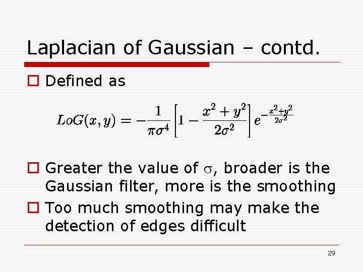
Laplacian of Gaussian – contd. o Defined as o Greater the value of s, broader is the Gaussian filter, more is the smoothing o Too much smoothing may make the detection of edges difficult 29

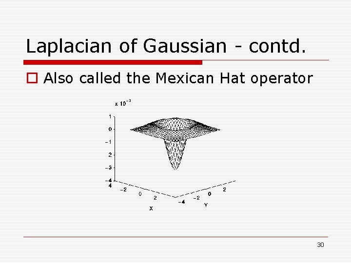
Laplacian of Gaussian - contd. o Also called the Mexican Hat operator 30

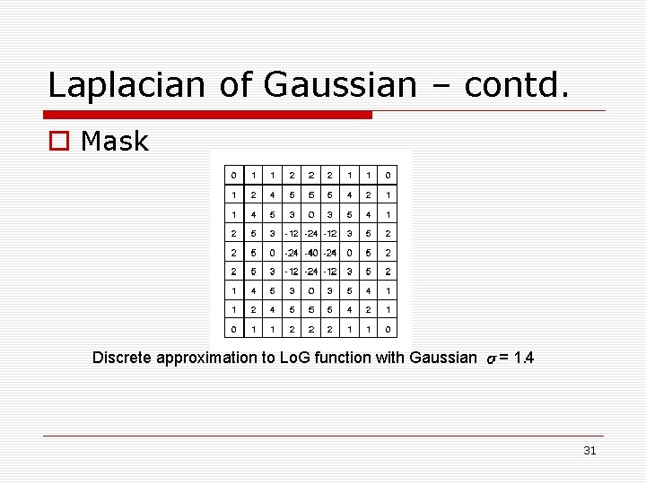
Laplacian of Gaussian – contd. o Mask Discrete approximation to Lo. G function with Gaussian = 1. 4 31

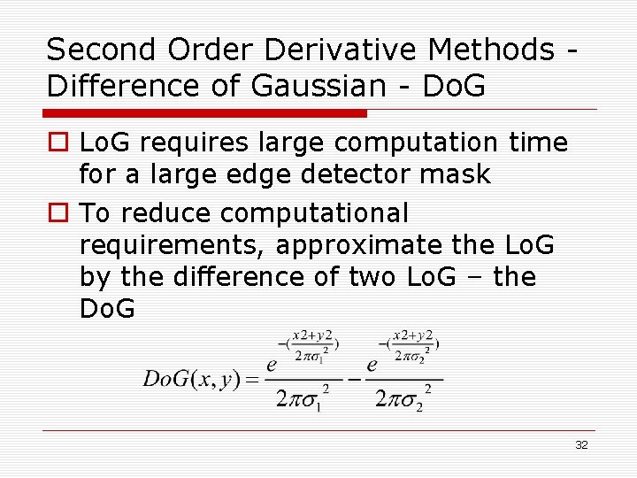
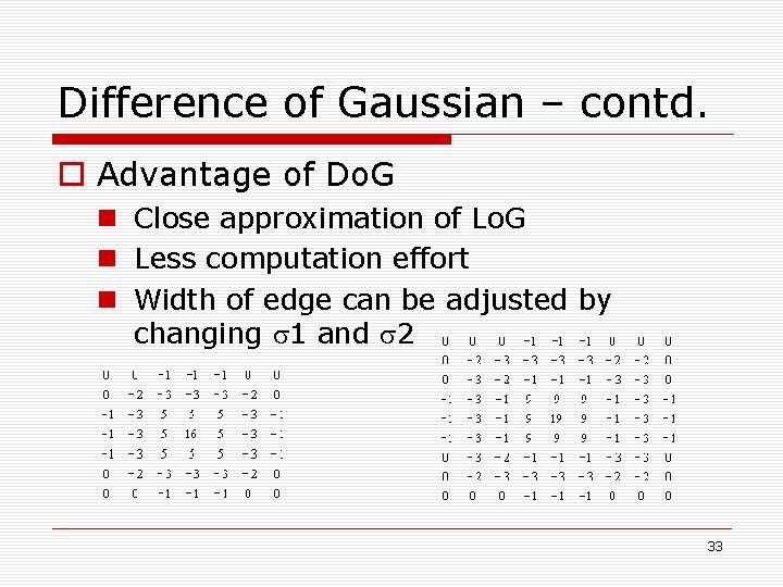
Second Order Derivative Methods Difference of Gaussian - Do. G o Lo. G requires large computation time for a large edge detector mask o To reduce computational requirements, approximate the Lo. G by the difference of two Lo. G – the Do. G 32

Difference of Gaussian – contd. o Advantage of Do. G n Close approximation of Lo. G n Less computation effort n Width of edge can be adjusted by changing s 1 and s 2 33

Second Order Derivative Methods Summary o Second Order Derivative methods especially Laplacian, are very sensitive to noise o Probability of false and missing edges remain o Localization is better than Gradient Operators 34

Optimal Edge Detector o Optimal edge detector depending on n Low error rate – edges should not be missed and there must not be spurious responses n Localization – distance between points marked by the detector and the actual center of the edge should be minimum n Response – Only one response to a single edge o One dimensional formulation n Assume that 2 D images have constant cross section in some direction 35

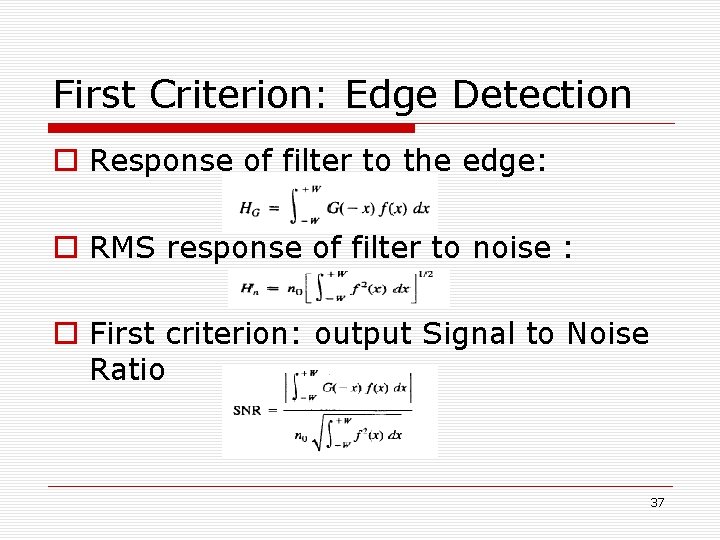
Mathematical Formulation of Performance Criteria o Notation n Edge : G(x) n Noise : n(x) n Impulse response of Filter : f(x) o Assumptions n n The edge is located at x=0 Filter has finite response bounded by [-W, W] Noise is of Gaussian nature n 0 : Root mean squared noise amplitude per unit length 36

First Criterion: Edge Detection o Response of filter to the edge: o RMS response of filter to noise : o First criterion: output Signal to Noise Ratio 37

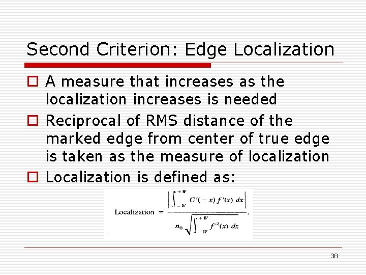
Second Criterion: Edge Localization o A measure that increases as the localization increases is needed o Reciprocal of RMS distance of the marked edge from center of true edge is taken as the measure of localization o Localization is defined as: 38

Maximizing the product o The design problem is reduced to maximization of the product: 39

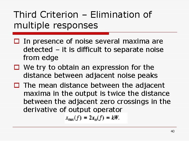
Third Criterion – Elimination of multiple responses o In presence of noise several maxima are detected – it is difficult to separate noise from edge o We try to obtain an expression for the distance between adjacent noise peaks o The mean distance between the adjacent maxima in the output is twice the distance between the adjacent zero crossings in the derivative of output operator 40

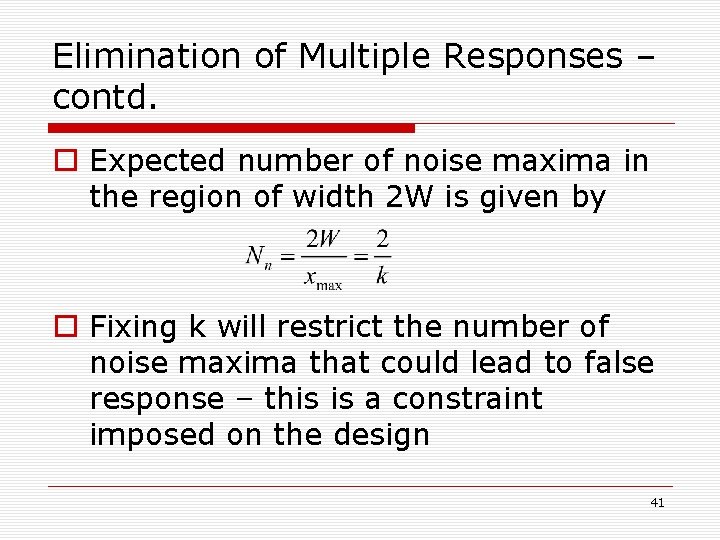
Elimination of Multiple Responses – contd. o Expected number of noise maxima in the region of width 2 W is given by o Fixing k will restrict the number of noise maxima that could lead to false response – this is a constraint imposed on the design 41

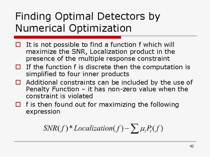
Finding Optimal Detectors by Numerical Optimization o It is not possible to find a function f which will maximize the SNR, Localization product in the presence of the multiple response constraint o If the function f is discrete then the computation is simplified to four inner products o Additional constraints can be included by the use of Penalty Function – it has non-zero value when the constraint is violated o f is then found out for maximizing the following expression 42

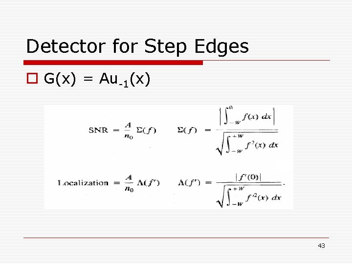
Detector for Step Edges o G(x) = Au-1(x) 43

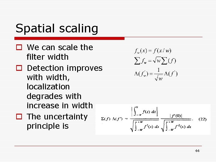
Spatial scaling o We can scale the filter width o Detection improves with width, localization degrades with increase in width o The uncertainty principle is 44

Efficient approximation o Depending on the above principles, several optimal edge detectors are calculated o Best approximation to the above detectors is the First Derivative of Gaussian o It is chosen because of the ease of computation in 2 dimensions 45

Noise estimation o Important to estimate the amount of noise in the image to set thresholds o Noise component can be efficiently isolated using Weiner Filtering – requires the knowledge of the autocorrelation of individual components and their crosscorrelation o Noise strength is estimated by Global Histogram Estimation 46

Thresholding o Broken edges due to fluctuation of operator output above and below the threshold – results in Streaking o Use double thresholding to eliminate streaking 47

Two Dimensional Edge Detection o In two dimensions edge has both position and direction o A 2 -D mask is created by convolving a linear edge detection function aligned normal to the edge direction with a projection function parallel the edge direction o Projection function is Gaussian with same deviation as the detection function o The image is convolved with a symmetric 2 D Gaussian and then differentiated normal to the edge direction 48

Need for multiple widths and Feature Synthesis o Width is chosen to give best tradeoff between detection and localization o For different edges, width has to be different since SNR is different o Feature Synthesis n Smaller operator responses are used to predict the larger operator response n New edge points are marked if the actual large operator output varies significantly from the predicted output 49

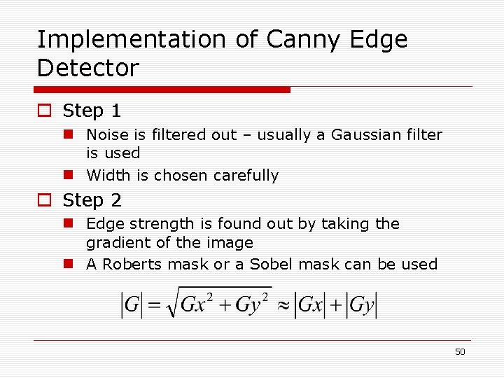
Implementation of Canny Edge Detector o Step 1 n Noise is filtered out – usually a Gaussian filter is used n Width is chosen carefully o Step 2 n Edge strength is found out by taking the gradient of the image n A Roberts mask or a Sobel mask can be used 50

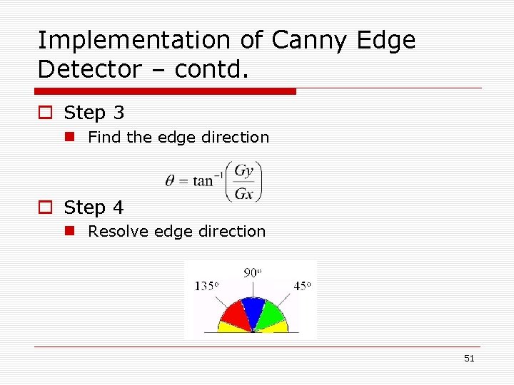
Implementation of Canny Edge Detector – contd. o Step 3 n Find the edge direction o Step 4 n Resolve edge direction 51

Canny Edge Detector – contd. o Step 5 n Non-maxima suppression – trace along the edge direction and suppress any pixel value not considered to be an edge. Gives a thin line for edge o Step 6 n Use double / hysterisis thresholding to eliminate streaking 52

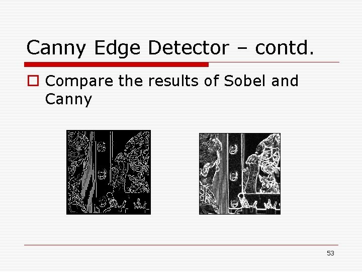
Canny Edge Detector – contd. o Compare the results of Sobel and Canny 53

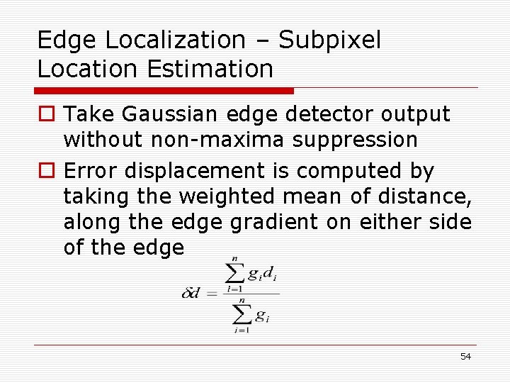
Edge Localization – Subpixel Location Estimation o Take Gaussian edge detector output without non-maxima suppression o Error displacement is computed by taking the weighted mean of distance, along the edge gradient on either side of the edge 54

Edge Detector Performance o Criteria Probability of false edges Probability of missing edges Error in estimation of edge angle Mean square distance of edge estimate from true edge n Tolerance to distorted edges and other features such as corners and junctions n n 55

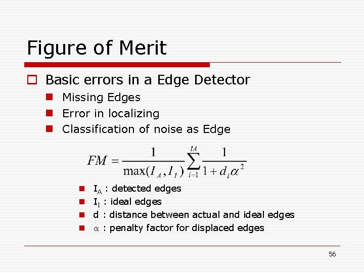
Figure of Merit o Basic errors in a Edge Detector n Missing Edges n Error in localizing n Classification of noise as Edge n n IA : detected edges II : ideal edges d : distance between actual and ideal edges a : penalty factor for displaced edges 56

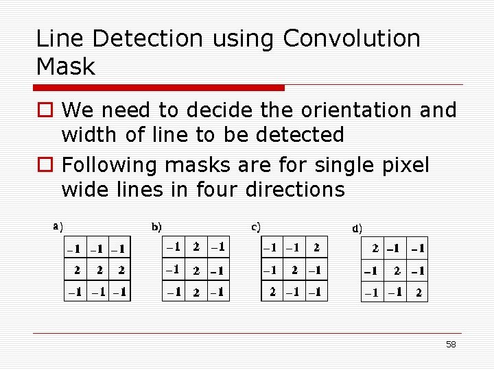
Line Detection o Lines in an image present another form of discontinuity o It is worthwhile to consider them separately since they are very frequent o Methods n Use of Convolution Mask n Hough Transform 57

Line Detection using Convolution Mask o We need to decide the orientation and width of line to be detected o Following masks are for single pixel wide lines in four directions 58

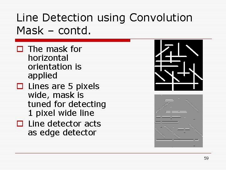
Line Detection using Convolution Mask – contd. o The mask for horizontal orientation is applied o Lines are 5 pixels wide, mask is tuned for detecting 1 pixel wide line o Line detector acts as edge detector 59

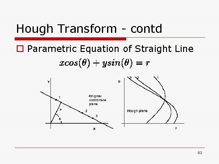
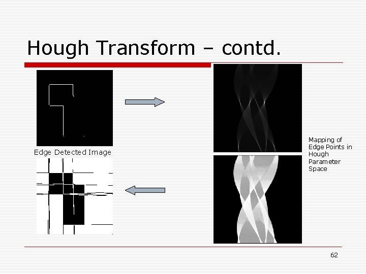
Line detection – Hough Transform o o Method to isolate the shapes from an image Performed after edge detection Not affected by noise or gaps in the edges Technique n Thresholding is used to isolate pixels with strong edge gradient n Parametric equation of straight line is used to map the edge points to the Hough parameter space n Points of intersection in the Hough parameter space gives the equation of line on actual image 60

Hough Transform - contd o Parametric Equation of Straight Line 61

Hough Transform – contd. Edge Detected Image Mapping of Edge Points in Hough Parameter Space 62

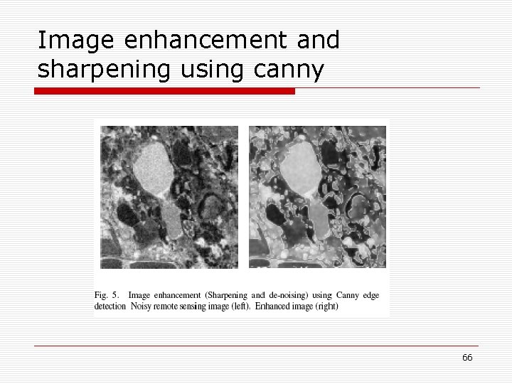
Applications o Enhancement of noisy images – satellite images, x-rays, medical images like cat scans o Text detection o Mapping of roads o Video surveillance, etc. 63

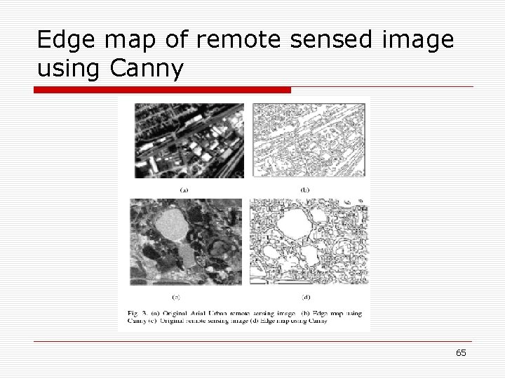
Applications o Canny Edge Detector for Remote Sensing Images n Reasons to go for Canny Edge Detector – Remote sensed images are inherently noisy n Other edge detectors are very sensitive to noise 64

Edge map of remote sensed image using Canny 65

Image enhancement and sharpening using canny 66

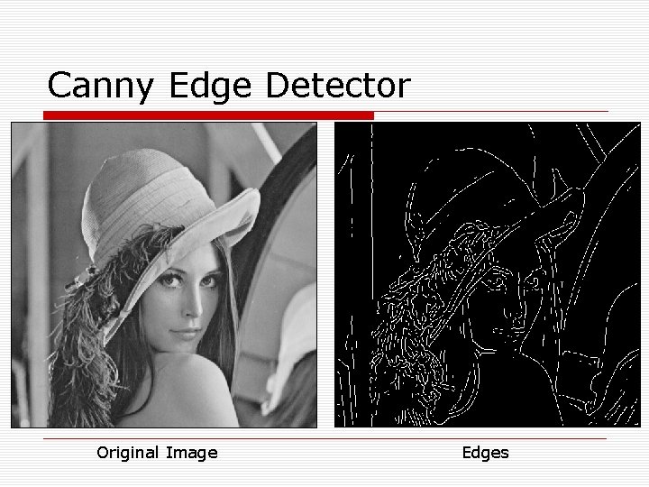
Canny Edge Detector Original Image Edges

MATLAB Demo o Get an image from the internet o Apply following operators on the image and display the results n n n Roberts Sobel Prewitt Laplacian of Gaussian Canny 68