Edge Detection Computer Vision P Schrater Spring 2003

Edge Detection Computer Vision P. Schrater Spring 2003

Simplest Model: (Canny) Edge(x) = a U(x) + n(x) ? U(x) x=0 Convolve image with U and find points with high magnitude. Choose value by comparing with a threshold determined by the noise model.

Probability of a filter response off an edge Probability of a filter response on an edge

Fundamental limits on edge detection

Need to take into account base edge rate.

Smoothing and Differentiation • Issue: noise – smooth before differentiation – two convolutions to smooth, then differentiate? – actually, no - we can use a derivative of Gaussian filter • because differentiation is convolution, and convolution is associative

There are three major issues: 1) The gradient magnitude at different scales is different; which should we choose? 2) The gradient magnitude is large along thick trail; how do we identify the significant points? 3) How do we link the relevant points up into curves?

1 pixel 3 pixels 7 pixels The scale of the smoothing filter affects derivative estimates, and also the semantics of the edges recovered.

Computing Edges via the gradient

We wish to mark points along the curve where the magnitude is biggest. We can do this by looking for a maximum along a slice normal to the curve (non-maximum suppression). These points should form a curve. There are then two algorithmic issues: at which point is the maximum, and where is the next one?

Non-maximum suppression At q, we have a maximum if the value is larger than those at both p and at r. Interpolate to get these values.

Predicting the next edge point Assume the marked point is an edge point. Then we construct the tangent to the edge curve (which is normal to the gradient at that point) and use this to predict the next points (here either r or s).

Remaining issues • Check that maximum value of gradient value is sufficiently large – drop-outs? use hysteresis • use a high threshold to start edge curves and a low threshold to continue them.

Edge Detection Algorithm • Define Edge filter: G= Dx = • Next Compute Gradient – Gradient Magnitude Gradient Direction

Edge Detection Algorithm • Find an initial point (i, j) such that: Where c is relatively large • Find nearby points in the direction of (i, j)’s gradient

Edge Detection Algorithm • While set of (i, j) with not visited – Find a start point, erasing points that have been checked. • While possible, expand a chain through the current point by: – 1) predicting a next set of points (not visited) using the direction perp. to gradient – 2) Finding which of set (if any) is a local maximum – 3) Test if grad mag for local max > k – 4) Recording all the set as visited • record point and set to current point. – end • end

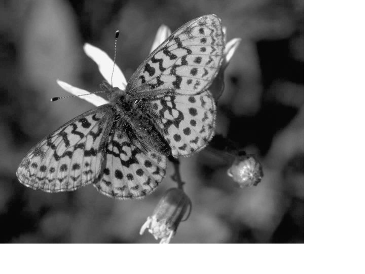
Notice • Something nasty is happening at corners • Scale affects contrast • Edges aren’t bounding contours

fine scale high threshold

coarse scale, high threshold

coarse scale low threshold

Positive responses Zero mean image, -1: 1 scale Zero mean image, -max: max scale

Positive responses Zero mean image, -1: 1 scale Zero mean image, -max: max scale

Figure from “Computer Vision for Interactive Computer Graphics, ” W. Freeman et al, IEEE Computer Graphics and Applications, 1998 copyright 1998, IEEE

The Laplacian of Gaussian • Another way to detect an extremal first derivative is to look for a zero second derivative • In 2 D: • Bad idea to apply a Laplacian without smoothing – smooth with Gaussian, apply Laplacian – this is the same as filtering with a Laplacian of Gaussian filter • Now mark the zero points where there is a sufficiently large derivative, and enough contrast

sigma=4 contrast=1 LOG zero crossings sigma=2 contrast=4

We still have unfortunate behaviour at corners

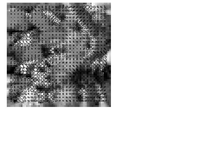
Orientation representations • The gradient magnitude is affected by illumination changes – but it’s direction isn’t • We can describe image patches by the swing of the gradient orientation • Important types: – constant window • small gradient mags – edge window • few large gradient mags in one direction – flow window • many large gradient mags in one direction – corner window • large gradient mags that swing

Representing Windows • Types – constant • small eigenvalues – Edge • one medium, one small – Flow • one large, one small – corner • two large eigenvalues

Filters are templates • Applying a filter at • Insight some point can be seen – filters look like the effects they are as taking a dot-product intended to find between the image and – filters find effects they some vector look like • Filtering the image is a set of dot products

Normalized correlation • Think of filters of a dot product – now measure the angle – i. e normalised correlation output is filter output, divided by root sum of squares of values over which filter lies • Tricks: – ensure that filter has a zero response to a constant region (helps reduce response to irrelevant background) – subtract image average when computing the normalizing constant (i. e. subtract the image mean in the neighbourhood) – absolute value deals with contrast reversal