ED International Trade Lecture 14 Giorgia Giovannetti Professor

E&D International Trade Lecture 14 Giorgia Giovannetti Professor of Economics, University of Firenze E-mail: giorgia. giovannetti@unifi. it

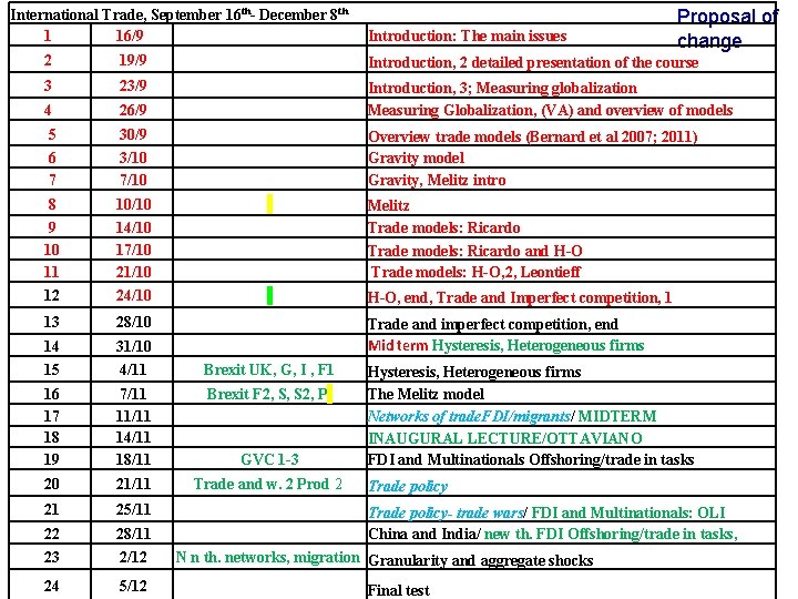
International Trade, September 16 th- December 8 th 1 16/9 Introduction: The main issues Proposal of change 2 19/9 Introduction, 2 detailed presentation of the course 3 23/9 4 26/9 Introduction, 3; Measuring globalization Measuring Globalization, (VA) and overview of models 5 30/9 6 7 3/10 7/10 8 10/10 9 10 11 14/10 17/10 21/10 12 Overview trade models (Bernard et al 2007; 2011) Gravity model Gravity, Melitz intro Melitz Trade models: Ricardo and H-O Trade models: H-O, 2, Leontieff 24/10 H-O, end, Trade and Imperfect competition, 1 13 28/10 14 31/10 Trade and imperfect competition, end Mid term Hysteresis, Heterogeneous firms 15 4/11 Brexit UK, G, I , F 1 16 17 18 19 7/11 11/11 14/11 18/11 Brexit F 2, S, S 2, P GVC 1 -3 20 21/11 Trade and w. 2 Prod 2 21 25/11 22 28/11 23 2/12 24 5/12 Hysteresis, Heterogeneous firms The Melitz model Networks of trade. FDI/migrants/ MIDTERM INAUGURAL LECTURE/OTTAVIANO FDI and Multinationals Offshoring/trade in tasks Trade policy- trade wars/ FDI and Multinationals: OLI China and India/ new th. FDI Offshoring/trade in tasks, N n th. networks, migration Granularity and aggregate shocks Final test

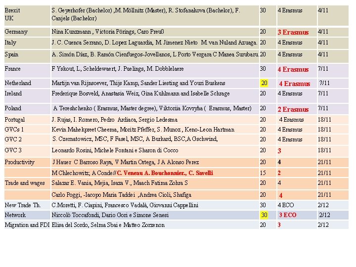
Brexit UK S. Geyerhofer (Bachelor) , M. Möllnitz (Master), R. Stofanakova (Bachelor), F. Canjels (Bachelor) 30 4 Erasmus 4/11 Germany Nina Kunzmann , Victoria Pörings, Caro Preuß 20 3 Erasmus 4/11 Italy J. C. Cuenca Serrano, D. Lopez Laguardia, M. Jimenez Nieto M. van Nuland Azuaga. 20 4 Erasmus 4/11 Spain A. Simón Díaz, B. Ramón Cienfuegos-Jovellanos, L Porto Vergara C Manea Surubaru. 20 4 Erasmus 4/11 France F Yskout, L, Scheldewaert, J. Puelings, M. Dobblelaere 30 4 Erasmus 7/11 Netherland Martijn van Rijnsoever, Thijs Kamp, Sander Liesting and Youri Buskens 20 4 Erasmus 7/11 Ireland Frederique Bosveld, Anastasia Weiz, Gina Kuhlmann and Isabelle Schrage 20 4 Erasmus 7/11 Poland A Tereshchenko ( Erasmus, Master degree), Viktoriia Kovryha ( Erasmus, Master) 20 2 Erasmus 7/11 Portugal J. Rujas, I. Romero, Pedro Ardiaca, Sergio Ledesma 20 4 Erasmus 18/11 GVCs 1 Kevin Mahekpreet Cheema, Moritz Pfeffer, S. Munoz , Keno-Leon Hartman 20 4 Erasmus 18/11 GVC 2 S. Czernatowicz, MSC, F Fasel, MSC, A Burkard, BSC, A Gschwind, 20 4 Erasmus 18/11 GVC 3 Leonardo Rosini, Michele Fontani e Sharon di Cocco 20 3 18/11 Productivity J Hauer C Barroso Raya, V Martin Ortega, J A Alonso Perez 20 4 21/11 M Chlechowitz; A Conde//C. Veneau A. Bouchonnier. , C. Savelli 15 2 21/11 Salazar E. Vania, Mejia, Isaza V. , Maach Fatima Zohra S 20 4 21/11 Carlo Poggi, -Iacopo Maria Taddei , Andrea Cioli, Shafiga 20 4 21/11 New Trade Th. C. Moretti, F. Ciapini, Francesco Vadalà, Giovanni Cappellini 30 4 ECO 2/12 Network Niccolò Toccafondi, Dario Gori e Simone Senesi 30 3 ECO 2/12 20 3 2/12 Trade and wages Migration and FDI Elisa del Sordo, Selma Sbai e Matteo Zorzenon

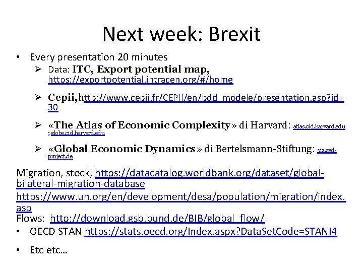
Next week: Brexit • Every presentation 20 minutes Ø Data: ITC, Export potential map, https: //exportpotential. intracen. org/#/home Ø Cepii, http: //www. cepii. fr/CEPII/en/bdd_modele/presentation. asp? id= 30 Ø «The Atlas of Economic Complexity» di Harvard: atlas. cid. harvard. edu ; globe. cid. harvard. edu Ø «Global Economic Dynamics» di Bertelsmann-Stiftung: viz. gedproject. de Migration, stock, https: //datacatalog. worldbank. org/dataset/globalbilateral-migration-database https: //www. un. org/en/development/desa/population/migration/index. asp Flows: http: //download. gsb. bund. de/BIB/global_flow/ • OECD STAN https: //stats. oecd. org/Index. aspx? Data. Set. Code=STANI 4 • Etc etc…

Articles that can be used for presentation on Brexit The latest on Brexit from the Decision Maker Panel, Nicholas Bloom, Philip Bunn, Scarlet Chen, Paul Mizen, Pawel Smietanka 25 September 2019, voxeu https: //voxeu. org/article/latest-brexit-decision-maker-panel • The impact of Brexit on UK firms, Nicholas Bloom, Philip Bunn, Scarlet Chen, Paul Mizen, Pawel Smietanka, Gregory Thwaites 04 September 2019 https: //voxeu. org/article/impact-brexit-uk-firms • EU-UK global value chain trade and the indirect costs of Brexit, Rita Cappariello, Michele Mancini, Filippo Vergara Caffarelli 22 March 2019 https: //voxeu. org/article/eu-uk-global-value-chain-trade-and-indirect-costs-brexit • Quantifying Brexit: From Ex Post to Ex Ante Using Structural Gravity, Felbermayr, Gabriel / Gröschl, Jasmin Katrin / Steininger, Marina, CESifo, Munich, 2018, Working Paper No. 7357 https: //www. cesifo. org/en/publikationen/2018/workingpaper/quantifying-brexit-ex-post-ex-ante-using-structural-gravity • Economic Effects of Brexit on the European Economy, Felbermayr, Gabriel / Fuest, Clemens / Gröschl, Jasmin Katrin / Stöhlker, Daniel, ifo Institute, Munich, 2017, Econ. Policy Report 4, https: //www. ifo. de/en/node/36858 Other readings on the web •

Where are we in Brexit?

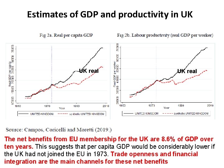
Estimates of GDP and productivity in UK UK real The net benefits from EU membership for the UK are 8. 6% of GDP over ten years. This suggests that per capita GDP would be considerably lower if the UK had not joined the EU in 1973. Trade openness and financial integration are the main channels for these net benefits

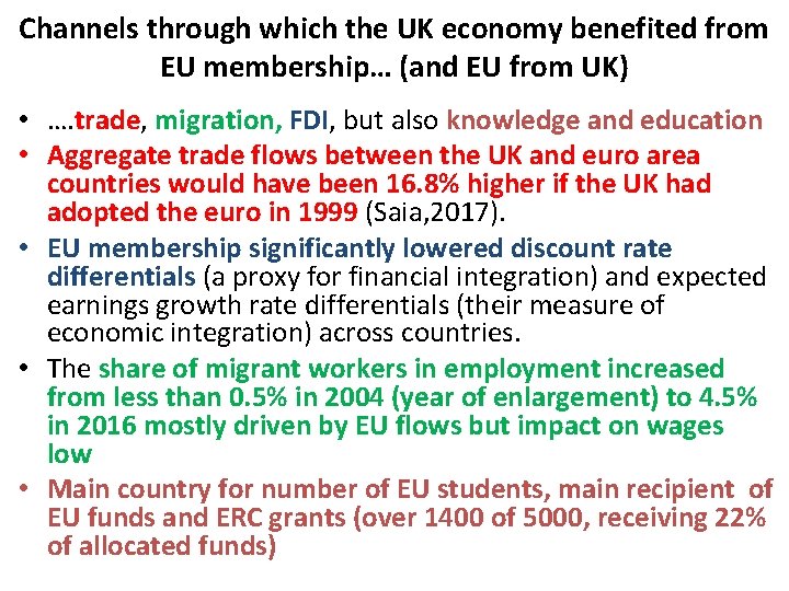
Channels through which the UK economy benefited from EU membership… (and EU from UK) • …. trade, migration, FDI, but also knowledge and education • Aggregate trade flows between the UK and euro area countries would have been 16. 8% higher if the UK had adopted the euro in 1999 (Saia, 2017). • EU membership significantly lowered discount rate differentials (a proxy for financial integration) and expected earnings growth rate differentials (their measure of economic integration) across countries. • The share of migrant workers in employment increased from less than 0. 5% in 2004 (year of enlargement) to 4. 5% in 2016 mostly driven by EU flows but impact on wages low • Main country for number of EU students, main recipient of EU funds and ERC grants (over 1400 of 5000, receiving 22% of allocated funds)

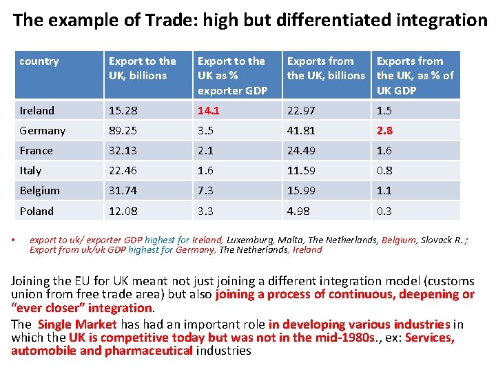
The example of Trade: high but differentiated integration • country Export to the UK, billions Export to the UK as % exporter GDP Exports from the UK, billions the UK, as % of UK GDP Ireland 15. 28 14. 1 22. 97 1. 5 Germany 89. 25 3. 5 41. 81 2. 8 France 32. 13 2. 1 24. 49 1. 6 Italy 22. 46 1. 6 11. 59 0. 8 Belgium 31. 74 7. 3 15. 99 1. 1 Poland 12. 08 3. 3 4. 98 0. 3 export to uk/ exporter GDP highest for Ireland, Luxemburg, Malta, The Netherlands, Belgium, Slovack R. ; Export from uk/uk GDP highest for Germany, The Netherlands, Ireland Joining the EU for UK meant not just joining a different integration model (customs union from free trade area) but also joining a process of continuous, deepening or “ever closer” integration. The Single Market has had an important role in developing various industries in which the UK is competitive today but was not in the mid-1980 s. , ex: Services, automobile and pharmaceutical industries

Clear? • Now back to imperfect competition models

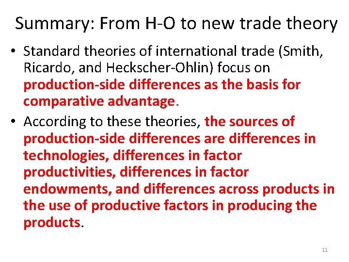
Summary: From H-O to new trade theory • Standard theories of international trade (Smith, Ricardo, and Heckscher-Ohlin) focus on production-side differences as the basis for comparative advantage. • According to these theories, the sources of production-side differences are differences in technologies, differences in factor productivities, differences in factor endowments, and differences across products in the use of productive factors in producing the products. 11

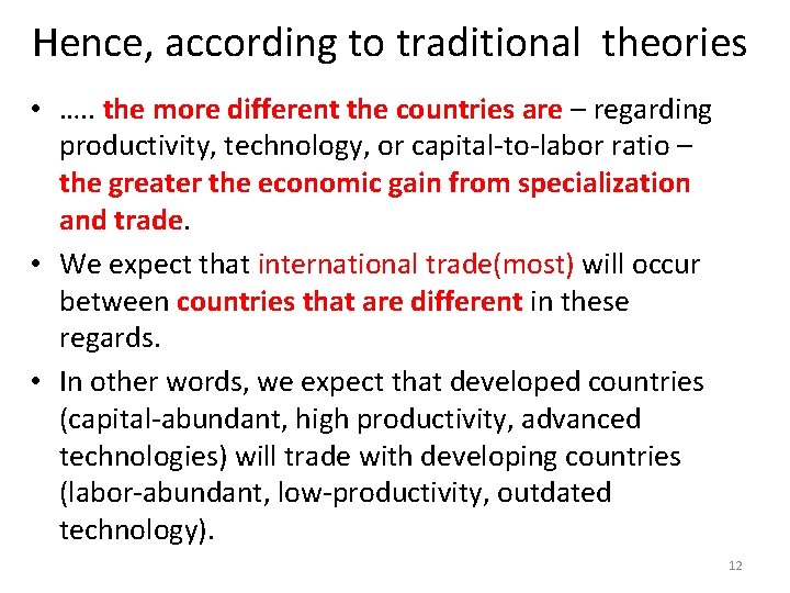
Hence, according to traditional theories • …. . the more different the countries are – regarding productivity, technology, or capital-to-labor ratio – the greater the economic gain from specialization and trade. • We expect that international trade(most) will occur between countries that are different in these regards. • In other words, we expect that developed countries (capital-abundant, high productivity, advanced technologies) will trade with developing countries (labor-abundant, low-productivity, outdated technology). 12

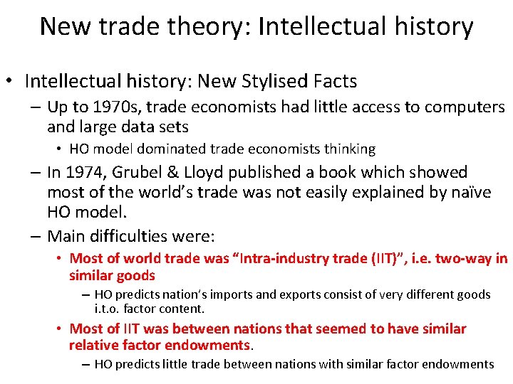
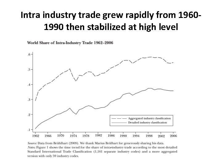
New trade theory: Intellectual history • Intellectual history: New Stylised Facts – Up to 1970 s, trade economists had little access to computers and large data sets • HO model dominated trade economists thinking – In 1974, Grubel & Lloyd published a book which showed most of the world’s trade was not easily explained by naïve HO model. – Main difficulties were: • Most of world trade was “Intra-industry trade (IIT)”, i. e. two-way in similar goods – HO predicts nation’s imports and exports consist of very different goods i. t. o. factor content. • Most of IIT was between nations that seemed to have similar relative factor endowments. – HO predicts little trade between nations with similar factor endowments

Intra industry trade grew rapidly from 19601990 then stabilized at high level

New Trade: Intellectual history (cont’d) • Grubel & Lloyd thought increasing returns to scale (IRS) were important. – Quite a number of non-mathematically economists knew about importance of IIT and had put forth informal analyses, most of which focused on IRS. – Basic idea was simple; trade occurs when things are made in one nation & consumed in another. IRS explains why production of particular goods is concentrated in a single nation rather than dispersed among all nations. This, plus the broad similarity of tastes among rich nations explains IIT.

New Trade: Intellectual history (cont’d) • At about same time, microeconomists developed tools for dealing with IRS in G. E. settings – Dixit-Stiglitz – Lancaster • In late 1970 s & early 1980 s, a few theorists showed that when IRS and/or Imperfect Competition (IC) was modeled in GE, IIT arose very naturally. – Krugman, Brander, Norman, Helpman, Markusen • This was the ‘new trade theory’ – It proved useful for understanding many aspects of the real world that ‘old trade theory’ (=Ricardo, Ricardo-Viner & HO) had to assume away due to Perfect Competition (PC) and Constant Returns to Scale (CRS). • Classical economists had many of the ideas but not the maths to crystallize the logic.

New Trade: Intellectual history (cont’d) • Pioneers: – Paul Krugman, articles in 1979, 1980, 1981. – Jim Brander, thesis in later 1970 s, articles in 1982, 84 (with Krugman) & strategic trade policy (with Barbara Spencer) in mid 1980 s. – Elhanan Helpman, articles in 1981 and books in 1985 & 1989 (with Krugman). MNCs in 1984. – Jim Markusen, articles in 1980 and on MNCs in 1984. – Many others.

Krugman model: basic idea • Ricardo, Ricardo-Viner & HO models all focus on differences between nations as a source of trade. • Krugman model focuses on geographical concentration of varieties. – Trade = made in one nation & purchased in another. • Internal IRS explains why production is concentrated geographically. • Resource constraints & IC explain why identical nations would each make some unique varieties. – One nation cannot make all (resource constraint). – Each firm makes unique variety to avoid direct competition. • Each nation makes some unique varieties, but buys some of every variety, so we see IIT between similar (even identical nations).

Trade facts in search of better theory 1. Substantial trade among industrialized countries, much of which is intraindustry trade. 2. The dominance of a few large firms in some world industries. We turn next to theories that focus not only on the supply side differences (technology, endowment, etc. ) but also on the demand side differences as the source of trade. 19

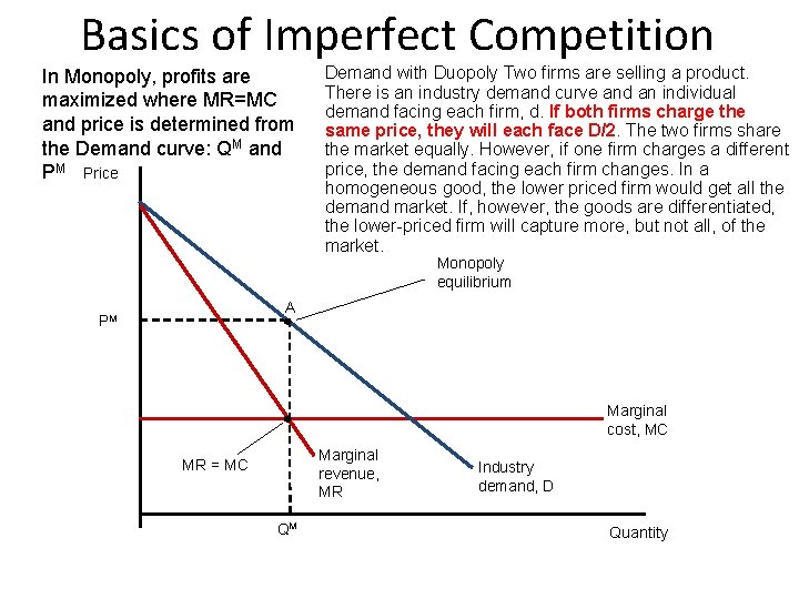
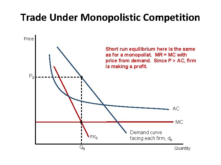
Basics of Imperfect Competition In Monopoly, profits are maximized where MR=MC and price is determined from the Demand curve: QM and PM Price Demand with Duopoly Two firms are selling a product. There is an industry demand curve and an individual demand facing each firm, d. If both firms charge the same price, they will each face D/2. The two firms share the market equally. However, if one firm charges a different price, the demand facing each firm changes. In a homogeneous good, the lower priced firm would get all the demand market. If, however, the goods are differentiated, the lower-priced firm will capture more, but not all, of the market. Monopoly equilibrium A PM Marginal cost, MC Marginal revenue, MR MR = MC QM Industry demand, D Quantity

Basics of Imperfect Competition • Demand with Duopoly – Since the goods are differentiated, some consumers will still choose to buy the higher price product. – The demand curve for the firm that lowered its price is flatter than the demand curve D/2 from before. – Each firm faces a more elastic demand curve than D/2, the curve it faces when the firms charge the same price.

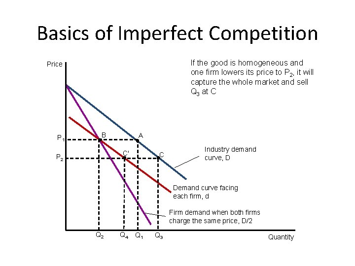
Basics of Imperfect Competition When arehomogeneous two firms in the If there good is and industry and both charge P , the If the goods are differentiated one firm lowers its price to 1 P 2, then it total will market demand is Q at A with each at P it will only capture part of the 1 2 capture the whole market and sell firm selling B 4 at C’ market 2 at Q Q 3 at C and. Qsell Price P 1 B A C' P 2 C Industry demand curve, D Demand curve facing each firm, d Firm demand when both firms charge the same price, D/2 Q 4 Q 1 Q 3 Quantity

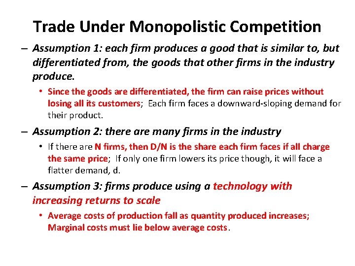
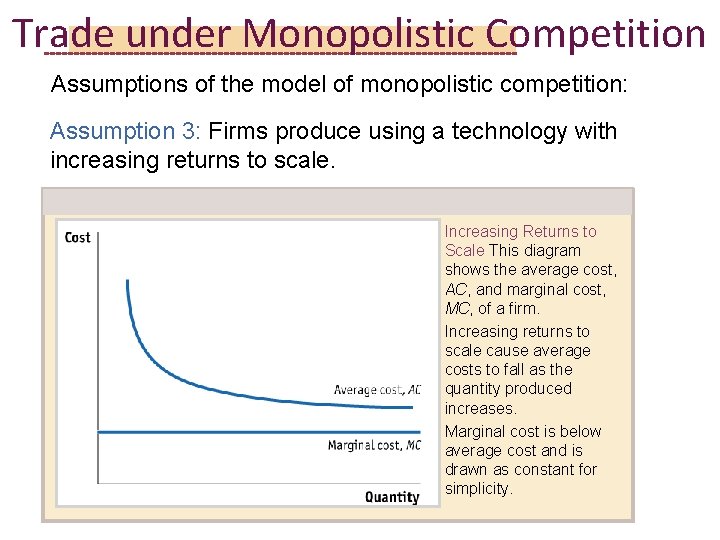
Trade Under Monopolistic Competition – Assumption 1: each firm produces a good that is similar to, but differentiated from, the goods that other firms in the industry produce. • Since the goods are differentiated, the firm can raise prices without losing all its customers; Each firm faces a downward-sloping demand for their product. – Assumption 2: there are many firms in the industry • If there are N firms, then D/N is the share each firm faces if all charge the same price; If only one firm lowers its price though, it will face a flatter demand, d. – Assumption 3: firms produce using a technology with increasing returns to scale • Average costs of production fall as quantity produced increases; Marginal costs must lie below average costs.

Trade under Monopolistic Competition Assumptions of the model of monopolistic competition: Assumption 3: Firms produce using a technology with increasing returns to scale. Increasing Returns to Scale This diagram shows the average cost, AC, and marginal cost, MC, of a firm. Increasing returns to scale cause average costs to fall as the quantity produced increases. Marginal cost is below average cost and is drawn as constant for simplicity.

Internal economies of scale • Scale economies are internal if the expansion of the size of the firm itself is the basis for the decline in its average cost. • Ways to reduce the average cost: – greater specialization of workers; – more specialized machines; – spreading of up-front fixed costs (R&D or production setup costs) over more units of output. 25

External economies of scale • Scale economies external to the individual firm relate to the size of the entire industry within a specific geographic area. • The average cost of the typical firm declines as the output of the industry in the area is larger. (Better input markets – specialized services and labor; swift diffusion of new knowledge about product and technology through direct contacts among the firms or as skilled workers transfer from firm to firm). 26

Trade Under Monopolistic Competition Price Short run equilibrium here is the same as for a monopolist. MR = MC with price from demand. Since P > AC, firm is making a profit. P 0 AC MC mr 0 Q 0 Demand curve facing each firm, d 0 Quantity

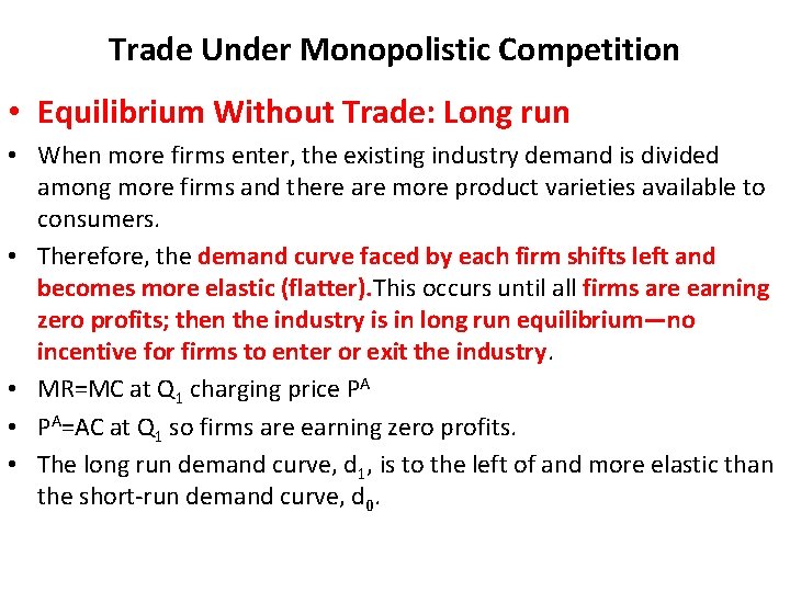
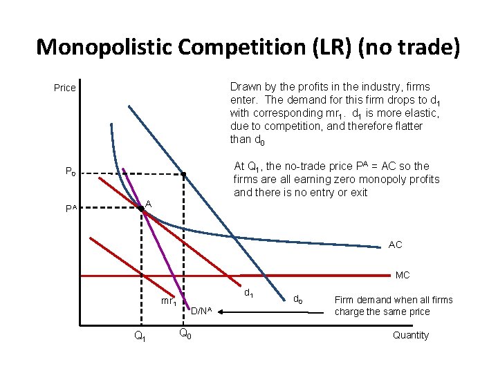
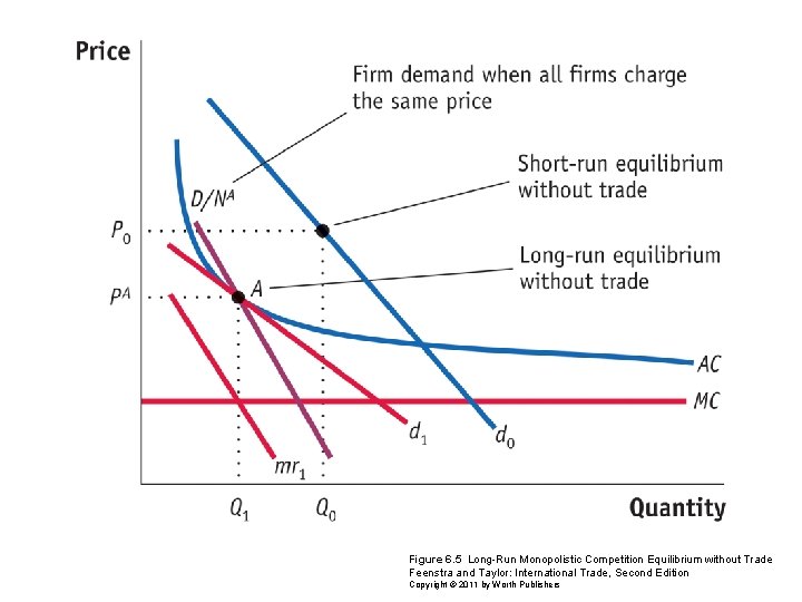
Trade Under Monopolistic Competition • Equilibrium Without Trade: Long run • When more firms enter, the existing industry demand is divided among more firms and there are more product varieties available to consumers. • Therefore, the demand curve faced by each firm shifts left and becomes more elastic (flatter). This occurs until all firms are earning zero profits; then the industry is in long run equilibrium—no incentive for firms to enter or exit the industry. • MR=MC at Q 1 charging price PA • PA=AC at Q 1 so firms are earning zero profits. • The long run demand curve, d 1, is to the left of and more elastic than the short-run demand curve, d 0.

Monopolistic Competition (LR) (no trade) Drawn by the profits in the industry, firms enter. The demand for this firm drops to d 1 Equilibrium is at A, producing Q 1, with corresponding mr 1. d 1 is more elastic, where mr 1 crosses MC. This gives due to competition, and therefore flatter price, PA, from the demand, d 1 than d 0 Price At Q 1, the no-trade price PA = AC so the firms are all earning zero monopoly profits and there is no entry or exit P 0 PA A AC MC mr 1 Q 1 d 1 D/NA Q 0 d 0 Firm demand when all firms charge the same price Quantity

Figure 6. 5 Long-Run Monopolistic Competition Equilibrium without Trade Feenstra and Taylor: International Trade, Second Edition Copyright © 2011 by Worth Publishers

Trade Under Monopolistic Competition – Hp: Home and Foreign are exactly the same. • Same number of consumers; Same technology and cost curves; Same number of firms in the no-trade equilibrium – If there were no economies of scale, there would be no reason for trade. • Under the Ricardian model, countries with identical technologies would not trade. • Under the Heckscher-Ohlin model, countries with identical factor endowments would not trade. • However, under monopolistic competition, two identical countries will still engage in trade.

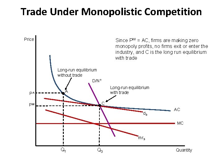
Long-Run Equilibrium with Trade – Since firms are making losses, some of them will go bankrupt and exit the industry. – The exit will increase demand for the remaining firms’ products and decrease the available product varieties to consumers. – We now only have NT firms which is fewer than the NA firms we had before. – The new demand D/NT lies to the right of D/NA. – Long-run equilibrium with trade is at point C. – The demand for each firm d 3 is tangent to AC.

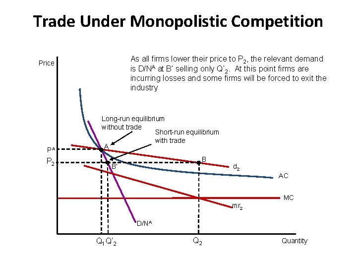
Short-Run Equilibrium with Trade – The number of firms in the no-trade equilibrium in each country is NA. Hp: each country is in long-run equilibrium without trade. When trade opens, the number of customers available to each firm doubles. – Since there are twice as many consumers, but also twice as many firms, the ratio stays the same. The product varieties also double. – With the greater number of varieties available, the demand for each individual variety will be more elastic. • If one firm drops its price below the no-trade price, it will get even more customers away from other firms; This gives demand curve, d 2, which is more elastic than the no-trade demand, d 1.

Trade & Monopolistic Competition – After trade, the new demand is no longer tangent to the AC. • Each firm now produces at Q 2 charging P 2 ; Firms are making positive monopoly profits; This shows the firm’s incentive to lower its price Short-Run Equilibrium with Trade – However, every firm in the industry has the same incentive— they can lower price and gain many more consumers and more profits. If all firms lower prices, the quantity demanded from each firm increases along D/NA, instead of d 2 (Remember D/NA is the demand if all firms had the same price). – In the short run, firms lower their prices expecting to make profits at B, but end up with losses at B′.

Trade Under Monopolistic Competition As all firms lower their the price to Pdemand Opening trade makes firm’s even more 2, the relevant A is D/N at B’ selling Q’firm this point are at Q 2, elastic, shown by d 2 only. The chooses to firms produce 2. At incurring losses and some forced exit the where MR=MC, selling at Pfirms thisbe price the to firm makes 2. Atwill industry monopoly profits as P 2>AC Price PA P 2 Long-run equilibrium without trade Short-run equilibrium with trade A B B’ d 2 AC MC mr 2 D/NA Q 1 Q’ 2 Quantity

Trade Under Monopolistic Competition Price Since some firms have exited the is Since PW = AC, firms making zero The demand faced byare each firm d 3 industry, are left T firms monopoly nowith firms exit orwhich enter the with mr 3 we. profits, mr 3=MC shows that each gives eachand firm. CQ aisshare of the Wequilibrium industry, the long rundemand firm produces 3 at a price P T shown by D/N with trade Long-run equilibrium without trade D/NT PA Long-run equilibrium with trade A C PW d 3 AC MC mr 3 Q 1 Q 3 Quantity

Comparison long-run equilibrium with trade versus equilibrium without trade – Even with the exit of some firms, we still expect that the world number of products is greater than the number available in each country before trade. – The demand curve facing each firm after trade is more elastic than the one before trade. – Fewer firms remain in each country, but each is bigger (i. e. there is an increase in quantity sold by each). – As quantity increases, average costs fall due to increasing returns to scale, therefore so do prices.

Sources of gains for consumers – Two : Price is lower after trade (due to the increased productivity for surviving firms due to increasing returns to scale); Consumers obtain higher surplus when there are more product varieties from which to choose. Although there are fewer product varieties made within each country (by fewer firms), consumers have more product variety because they can choose products from the firms of both countries. • Adjustment Costs from Trade – There adjustment costs as some firms shut down and exit the industry. – Workers in those firms experience unemployment. – Over the long run however, we expect those workers to find new positions. Hence the costs are temporary

Summary: Monopolistic Competition Implications – Trade gains through “new products” consumed – Model explains intra-industry trade – Product-differentiated bilateral exports remain positive from any country that produces - less sensitive to trade costs – Model has a role for firms – in form of a representative firm

Summary: new trade theory • Introduced increasing returns, imperfect competition and product differentiation – This helped resolve the indeterminacy of firm size – With product differentiation, firms face downward sloping demand curves and there exists an optimal firm size • Free entry (and general equilibrium) then pins down industry size and also the number of firms within an industry • New Trade Theory rationalized two-way trade flows in similar products across countries

Demand & Product differentiation • Growth in intra-industry trade over time and higher intra-industry trade for higherincome countries can be understood partly from the demand side. • Income growth shifts demand toward luxuries, and product variety is a luxury. Affluent people vary their choices of wines, beers, automobiles, music, clothing, travel expenses, and so on. 41

• Full customization of production in a single country would be too costly. • Hence, some varieties will be imported, while the varieties produced in the country can be exported to affluent consumers in other countries. • When all firms face similar downwardsloping average cost curves, so there may be no comparative advantage. • Rather, a country’s trade is based on product differentiation. 42

• The basis for exporting is the domestic production of unique models (or varieties) demanded by some consumers in foreign markets. • The basis for importing is the demand by some domestic consumers for unique models produced by foreign firms. • Intra-industry trade in different products can be large, even between countries that are similar in their general production capabilities. 43

Economies of scale • Yet, demand effects cannot be the whole story. • Economies of scale play a supporting role, by encouraging production specialization for different varieties. • With trade, firms in each country produce only a limited number of varieties of the basic product, but in greater quantities (domestic market + exports), which leads to a lower unit production costs. 44

• If internal scale economies are modest or moderate, then there is room in the industry for a large number of firms. If, in addition, products are differentiated, then we have a mild form of imperfect competition called monopolistic competition. 45

• If internal scale economies are substantial over a large range of output, then it is likely that a few firms will grow to be large in order to reap the scale economies. If a few large firms dominate the global industry, then we have an oligopoly. • The countries in which these firms are located will then tend to be net exporters of the product, while other countries are importers. 46

• External scale economies appear to explain the clustering of some industries: • Silicon Valley – high-tech semiconductor, computer, and related producers. • New York City – banking and finance. • Hollywood (Bollywood in Bombay) – filmmaking. • Italy – stylish clothing, shoes, and accessories. • Switzerland – watches. 47

Gains from trade • A major additional source of national gains from trade is the increase in the number of varieties of products that become available to consumers through imports. • Without trade, nations might not be able to produce those products where economies of scale are important. With trade, markets are large enough to support the production necessary to achieve economies of scale. 48

Implications of new trade theory • Nations may benefit from trade even when they do not differ in resource endowments or technology. • The theory does not contradict comparative advantage theory, but instead identifies a source of comparative advantage. • Governments should consider strategic trade policies that nurture and protect firms and industries where first mover advantages and economies of scale are important. 49

Some Problematic Predictions of the new theory • As insightful as New Trade Theory is, it delivers some counterfactual predictions • Because all firms within a sector are treated symmetrically, either all firms within an industry export or none does (and they always do with CES) • Trade liberalization generally affects all firms within an industry symmetrically (and when it doesn’t, there is no way to predict these asymmetries) • This is NOT a good description of reality

Criticism of new trade theory 1. The monopolistic-competition model suggests that product differentiation can be a basis for successful exporting, although it does not predict which specific varieties of a differentiated product will be produced by which country. 51

Similarity = Trade • Even identical countries may trade • This could happen simply because their technologies may have increasing returns to scale (IRS) • As a result of trade, the number of firms in a new international industry is predicted to increase relative to each national market. – But it is unclear if firms will locate in the domestic country or foreign countries.

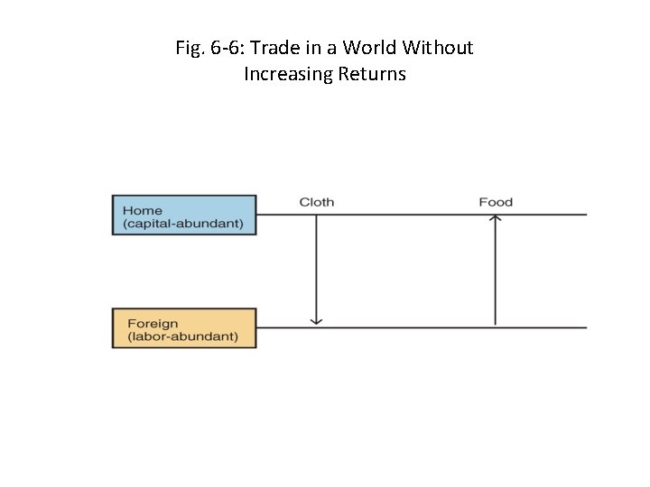
Inter-industry Trade • According to the Heckscher-Ohlin model or Ricardian model, countries specialize in production. – Trade occurs only between industries: inter-industry trade • In a Heckscher-Ohlin model suppose that: – The capital abundant domestic economy specializes in the production of capital intensive cloth, which is imported by the foreign economy. – The labor abundant foreign economy specializes in the production of labor intensive food, which is imported by the domestic economy.

Fig. 6 -6: Trade in a World Without Increasing Returns

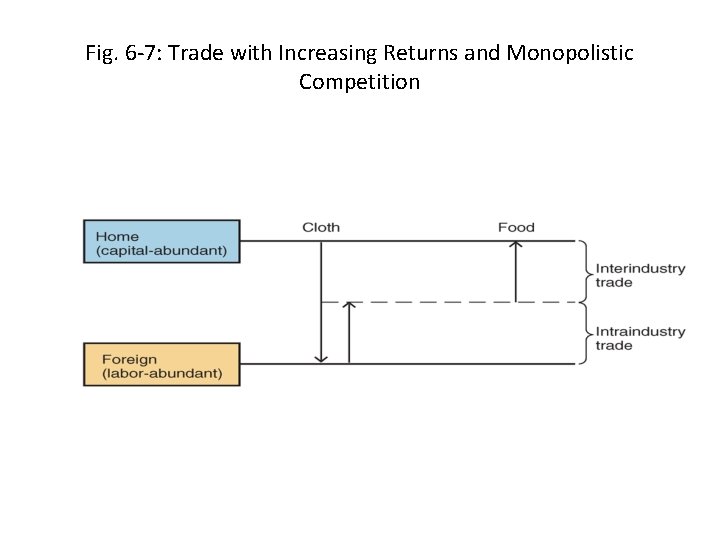
Intra-industry Trade • Suppose now that the global cloth industry is described by the monopolistic competition model. • Because of product differentiation, suppose that each country produces different types of cloth. • Because of economies of scale, large markets are desirable: the foreign country exports some cloth and the domestic country exports some cloth. – Trade occurs within the cloth industry: intra-industry trade • If domestic country is capital abundant, it still has a comparative advantage in cloth. – It should therefore export more cloth than it imports. • Suppose that the trade in the food industry continues to be determined by comparative advantage.

Fig. 6 -7: Trade with Increasing Returns and Monopolistic Competition

Inter-industry and Intra-industry Trade 1. Gains from inter-industry trade reflect comparative advantage. 2. Gains from intra-industry trade reflect economies of scale (lower costs) and wider consumer choices. 3. The monopolistic competition model does not predict in which country firms locate, but a comparative advantage in producing the differentiated good will likely cause a country to export more of that good than it imports.

Inter-industry and Intra-industry Trade (cont. ) 4. The relative importance of intra-industry trade depends on how similar countries are. – Countries with similar relative amounts of factors of production are predicted to have intraindustry trade. – Countries with different relative amounts of factors of production are predicted to have interindustry trade. 5. Unlike inter-industry trade in the Heckscher-Ohlin model, income distribution effects are not predicted to occur with intra-industry trade.

Inter-industry and Intra-industry Trade (cont. ) • About 25% of world trade is intra-industry trade according to standard industrial classifications. – But some industries have more intra-industry trade than others: those industries requiring relatively large amounts of skilled labor, technology, and physical capital exhibit intra-industry trade for the U. S. – Countries with similar relative amounts of skilled labor, technology, and physical capital engage in a large amount of intra-industry trade with the U. S.