Economic Growth IV New Growth Evidence Gavin Cameron

Economic Growth IV: New Growth Evidence Gavin Cameron Lady Margaret Hall Hilary Term 2004

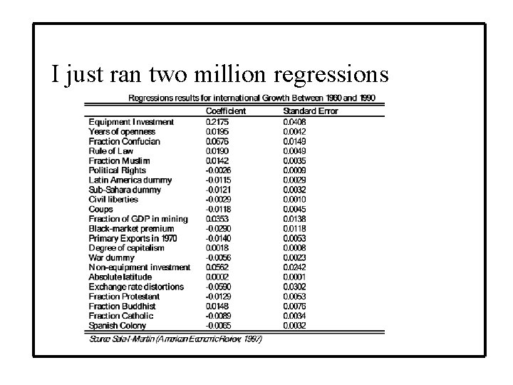
new growth evidence • This lecture surveys the evidence on economic growth performance across the world. It examines four issues: • Development as Freedom, Growth Miracles and Disasters: • Does growth matter? Who has done well and badly? • Growth Accounting, R&D Accounting and Standing on Shoulders: • How can you account for growth? • Convergence, Galton’s Fallacy and Twin Peaks; • Do countries converge? How can you measure convergence? • Two Million Regressions and the Correlates of High Income. • What factors are correlated with rapid growth and high income?

development as freedom • ‘Development can be seen…as a process of expanding the real freedoms that people enjoy. ’ Amartya Sen, Development as Freedom, 2000. • Political freedom, such as the ability to choose who governs and how they do so and to be able to write and speak freely. • Economic freedom, such as the ability to consume, produce and exchange, and to do rewarding work. • Social opportunities, such as the provision of public goods like healthcare and education. • Transparency guarantees, such as clear and truthful information about current affairs and politics, and what is being offered to whom. • Protective security, such as protection against risks like unemployment, crime, famine and war.

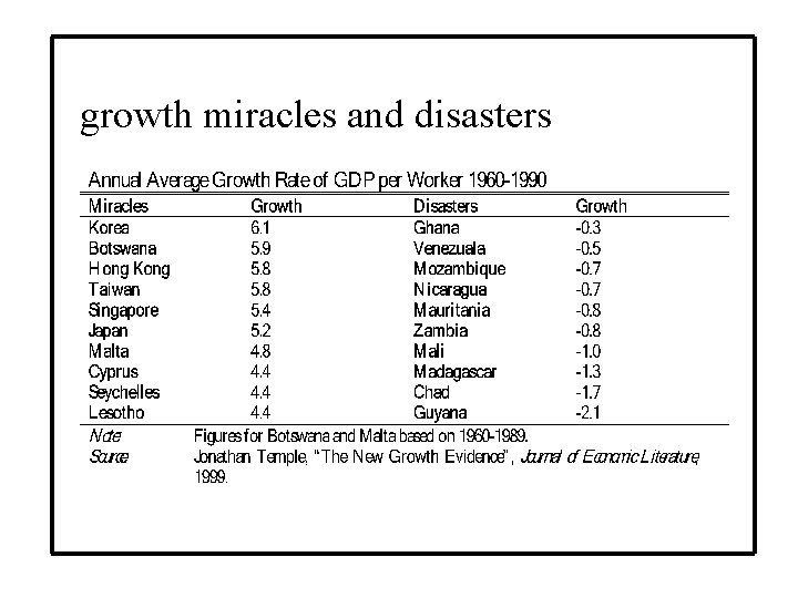
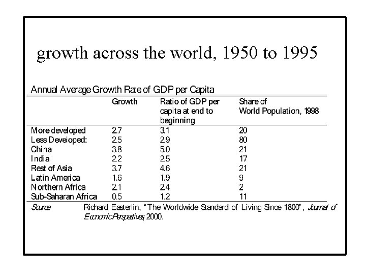
growth miracles and disasters

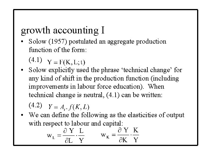
growth accounting I • Solow (1957) postulated an aggregate production function of the form: (4. 1) • Solow explicitly used the phrase ‘technical change’ for any kind of shift in the production function (including improvements in labour force education). When technical change is neutral, (4. 1) can be written: (4. 2) • We can define the following as the elasticities of output with respect to labour and capital:

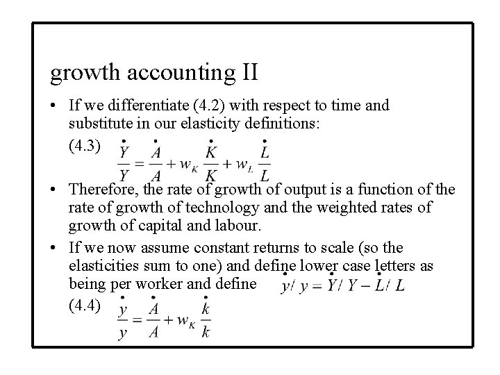
growth accounting II • If we differentiate (4. 2) with respect to time and substitute in our elasticity definitions: (4. 3) • Therefore, the rate of growth of output is a function of the rate of growth of technology and the weighted rates of growth of capital and labour. • If we now assume constant returns to scale (so the elasticities sum to one) and define lower case letters as being per worker and define (4. 4)

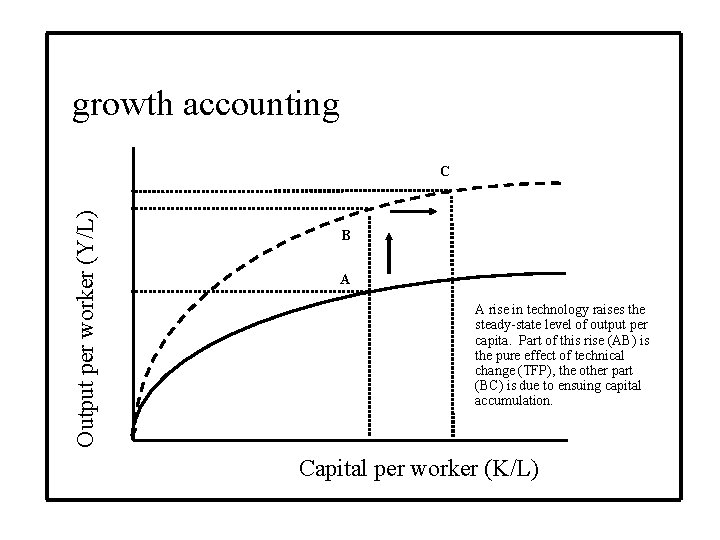
growth accounting Output per worker (Y/L) C B A A rise in technology raises the steady-state level of output per capita. Part of this rise (AB) is the pure effect of technical change (TFP), the other part (BC) is due to ensuing capital accumulation. Capital per worker (K/L)

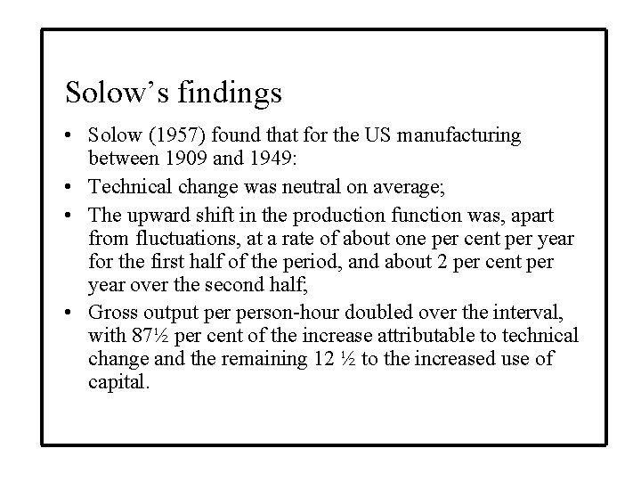
Solow’s findings • Solow (1957) found that for the US manufacturing between 1909 and 1949: • Technical change was neutral on average; • The upward shift in the production function was, apart from fluctuations, at a rate of about one per cent per year for the first half of the period, and about 2 per cent per year over the second half; • Gross output person-hour doubled over the interval, with 87½ per cent of the increase attributable to technical change and the remaining 12 ½ to the increased use of capital.

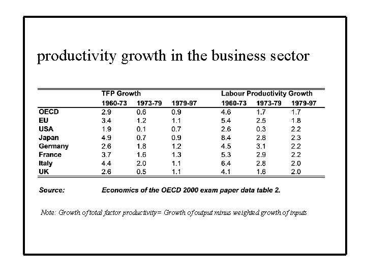
productivity growth in the business sector Note: Growth of total factor productivity= Growth of output minus weighted growth of inputs

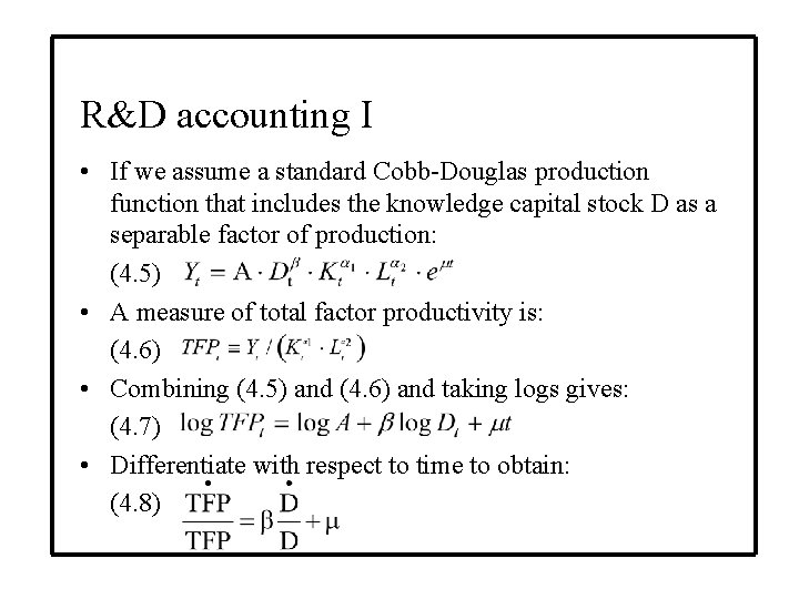
R&D accounting I • If we assume a standard Cobb-Douglas production function that includes the knowledge capital stock D as a separable factor of production: (4. 5) • A measure of total factor productivity is: (4. 6) • Combining (4. 5) and (4. 6) and taking logs gives: (4. 7) • Differentiate with respect to time to obtain: (4. 8)

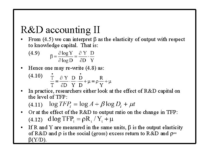
R&D accounting II • From (4. 5) we can interpret as the elasticity of output with respect to knowledge capital. That is: (4. 9) • Hence one may re-write (4. 8) as: (4. 10) • In practice, researchers either look at the effect of R&D capital on the level of TFP: (4. 11) • Or at the effect of the R&D to output ratio on the change in TFP: (4. 12) • If R and Y are measured in the same units, is the output elasticity of R&D and is the social (gross) excess return to R&D and = (Y/D).

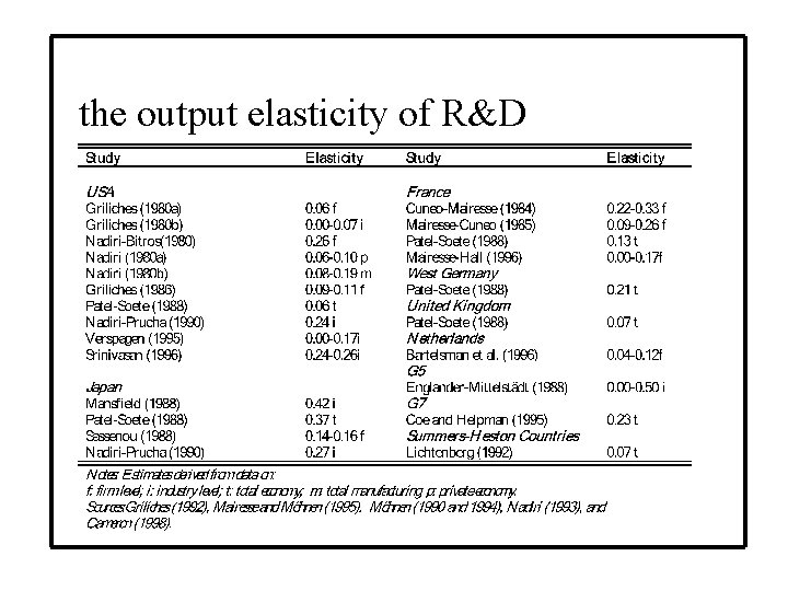
the output elasticity of R&D

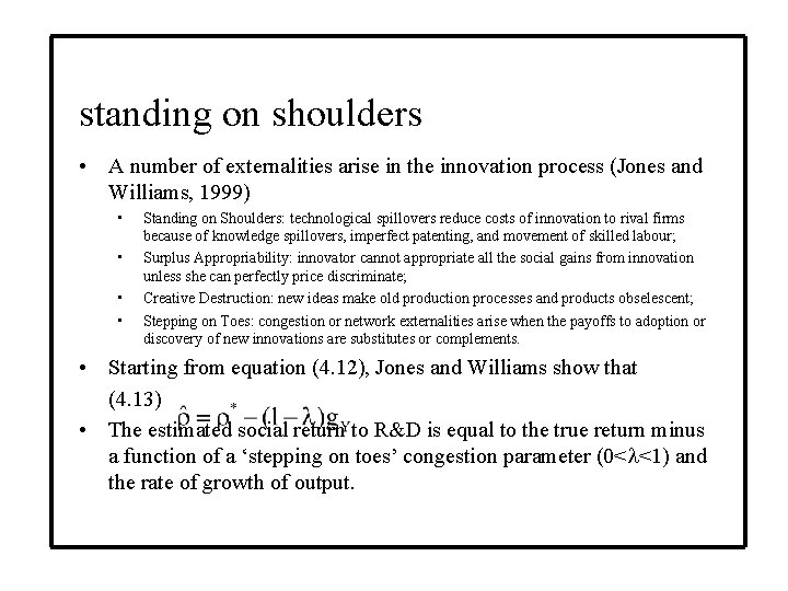
standing on shoulders • A number of externalities arise in the innovation process (Jones and Williams, 1999) • • Standing on Shoulders: technological spillovers reduce costs of innovation to rival firms because of knowledge spillovers, imperfect patenting, and movement of skilled labour; Surplus Appropriability: innovator cannot appropriate all the social gains from innovation unless she can perfectly price discriminate; Creative Destruction: new ideas make old production processes and products obselescent; Stepping on Toes: congestion or network externalities arise when the payoffs to adoption or discovery of new innovations are substitutes or complements. • Starting from equation (4. 12), Jones and Williams show that (4. 13) • The estimated social return to R&D is equal to the true return minus a function of a ‘stepping on toes’ congestion parameter (0< <1) and the rate of growth of output.

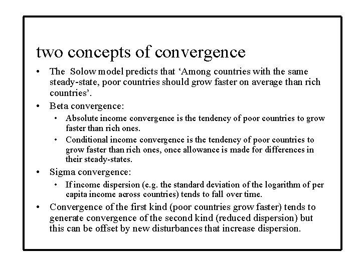
two concepts of convergence • The Solow model predicts that ‘Among countries with the same steady-state, poor countries should grow faster on average than rich countries’. • Beta convergence: • Absolute income convergence is the tendency of poor countries to grow faster than rich ones. • Conditional income convergence is the tendency of poor countries to grow faster than rich ones, once allowance is made for differences in their steady-states. • Sigma convergence: • If income dispersion (e. g. the standard deviation of the logarithm of per capita income across countries) tends to fall over time. • Convergence of the first kind (poor countries grow faster) tends to generate convergence of the second kind (reduced dispersion) but this can be offset by new disturbances that increase dispersion.

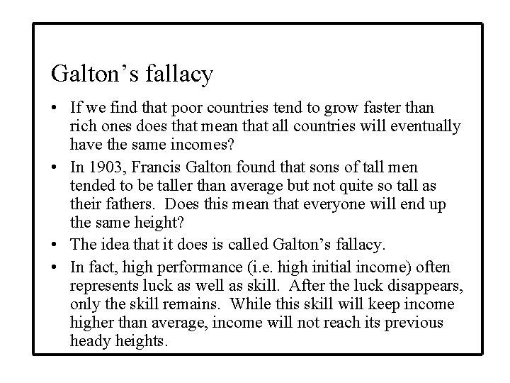
Galton’s fallacy • If we find that poor countries tend to grow faster than rich ones does that mean that all countries will eventually have the same incomes? • In 1903, Francis Galton found that sons of tall men tended to be taller than average but not quite so tall as their fathers. Does this mean that everyone will end up the same height? • The idea that it does is called Galton’s fallacy. • In fact, high performance (i. e. high initial income) often represents luck as well as skill. After the luck disappears, only the skill remains. While this skill will keep income higher than average, income will not reach its previous heady heights.

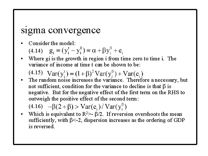
sigma convergence • Consider the model: (4. 14) • Where gi is the growth in region i from time zero to time i. The variance of income at time t can be shown to be: (4. 15) • The random noise increases the variance. Therefore a necessary, but not sufficient, condition for the variance to decline is that is negative. But for the negative effect of the first term on the RHS to outweigh the positive effect of the second term: (4. 16) • Which is equivalent to R 2>- /2. If reversion overshoots the mean sufficiently, with <-2, dispersion increases as the ordering of GDP is reversed.

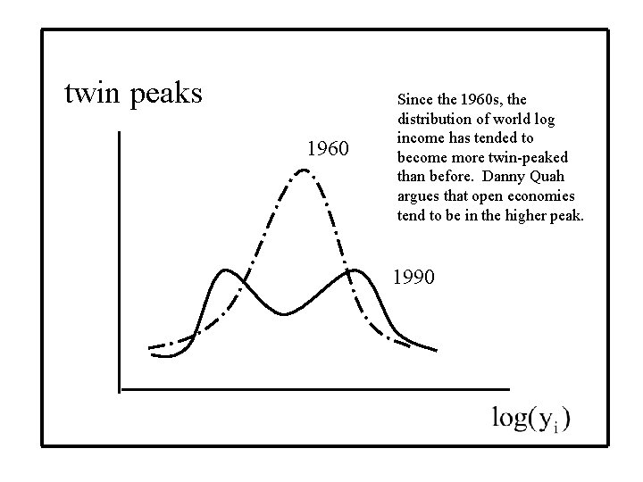
twin peaks 1960 Since the 1960 s, the distribution of world log income has tended to become more twin-peaked than before. Danny Quah argues that open economies tend to be in the higher peak. 1990

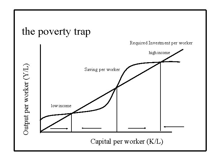
the poverty trap Required Investment per worker Output per worker (Y/L) high income Saving per worker low income Capital per worker (K/L)

I just ran two million regressions

growth across the world, 1950 to 1995

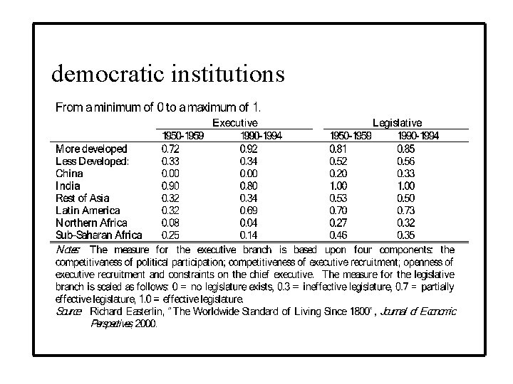
democratic institutions

total factor productivity • A typical worker in US or Switzerland is 20 to 30 times more productive than a worker in Haiti or Nigeria. • Between-country differences much greater than within-country differences. • Some of this can be explained by natural resources, oil. • Some can be explained by physical capital, but investment rates surprisingly similar across countries. • Nor can human capital explain differences, unless investments in intangibles much bigger than we think. • Therefore, differences in technology must matter. • What are the barriers to efficient adoption and use of technologies across the world?

high productivity countries • Institutions that favour production over diversion; • Low rate of government consumption (i. e. not investment or transfers); • Open to international trade; • Well-educated workforce; • Private ownership and good quality institutions; • International language; • Temperate latitude far from equator.