Econometrics Lecture 1 Introduction to Linear Regression Contents

Econometrics - Lecture 1 Introduction to Linear Regression

Contents n Organizational Issues Some History of Econometrics n An Introduction to Linear Regression n n q OLS as an algebraic tool q The Linear Regression Model q Small Sample Properties of OLS estimator Introduction to GRETL Sept 24, 2010 Hackl, Econometrics 2

Organizational Issues Aims of the course n Understanding of econometric concepts and principles n Introduction to commonly used econometric tools and techniques n Use of econometric tools for analyzing economic data: specification of adequate models, identification of appropriate econometric methods, interpretation of results n Use of GRETL Sept 24, 2010 Hackl, Econometrics 3

Organizational Issues, cont’d Literature Course textbook n Marno Verbeek, A Guide to Modern Econometrics, 3 rd Ed. , Wiley, 2008 Suggestions for further reading n P. Kennedy, A Guide to Econometrics, 6 th Ed. , Blackwell, 2008 n W. H. Greene, Econometric Analysis. 6 th Ed. , Pearson International, 2008 Sept 24, 2010 Hackl, Econometrics 4

Organizational Issues, cont’d Prerequisites n Linear algebra: linear equations, matrices, vectors (basic operations and properties) n Descriptive statistics: measures of central tendency, measures of dispersion, measures of association, histogram, frequency tables, scatter plot, quantile n Theory of probability: probability and its properties, random variables and distribution functions in one and several dimensions, moments, convergence of random variables, limit theorems, law of large numbers n Mathematical statistics: point estimation, confidence intervals, hypothesis testing, p-value, significance level Sept 24, 2010 Hackl, Econometrics 5

Organizational Issues, cont’d Teaching and learning method n Course in six blocks n Class discussion, written homework (computer exercises, GRETL) submitted by groups of (3 -5) students, presentations of homework by participants n Final exam Assessment of student work n For grading, the written homework, presentation of homework in class and a final written exam will be of relevance n Weights: homework 70 %, final written exam 30 % n Presentation of homework in class: students must be prepared to be called at random Sept 24, 2010 Hackl, Econometrics 6

Contents n Organizational Issues Some History of Econometrics n An Introduction to Linear Regression n n q OLS as an algebraic tool q The Linear Regression Model q Small Sample Properties of OLS estimator Introduction to GRETL Sept 24, 2010 Hackl, Econometrics 7

Empirical Economics Prior to 1930 ies The situation in the early 1930 ies: n Theoretical economics aims at “operationally meaningful theorems“; “operational” means purely logical mathematical deduction n Economic theories or laws are seen as deterministic relations; no inference from data as part of economic analysis n Ignorance of the stochastic nature of economic concepts n Use of statistical methods for q q n measuring theoretical coefficients, e. g. , demand elasticities, representing business cycles Data: limited availability; time-series on agricultural commodities, foreign trade Sept 24, 2010 Hackl, Econometrics 8

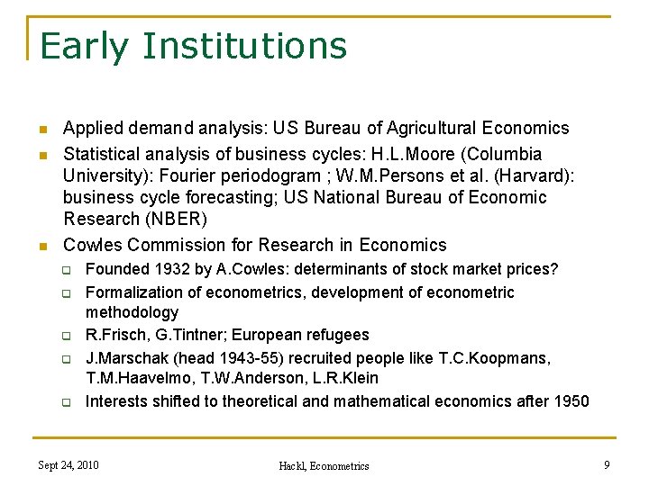
Early Institutions n n n Applied demand analysis: US Bureau of Agricultural Economics Statistical analysis of business cycles: H. L. Moore (Columbia University): Fourier periodogram ; W. M. Persons et al. (Harvard): business cycle forecasting; US National Bureau of Economic Research (NBER) Cowles Commission for Research in Economics q q q Founded 1932 by A. Cowles: determinants of stock market prices? Formalization of econometrics, development of econometric methodology R. Frisch, G. Tintner; European refugees J. Marschak (head 1943 -55) recruited people like T. C. Koopmans, T. M. Haavelmo, T. W. Anderson, L. R. Klein Interests shifted to theoretical and mathematical economics after 1950 Sept 24, 2010 Hackl, Econometrics 9

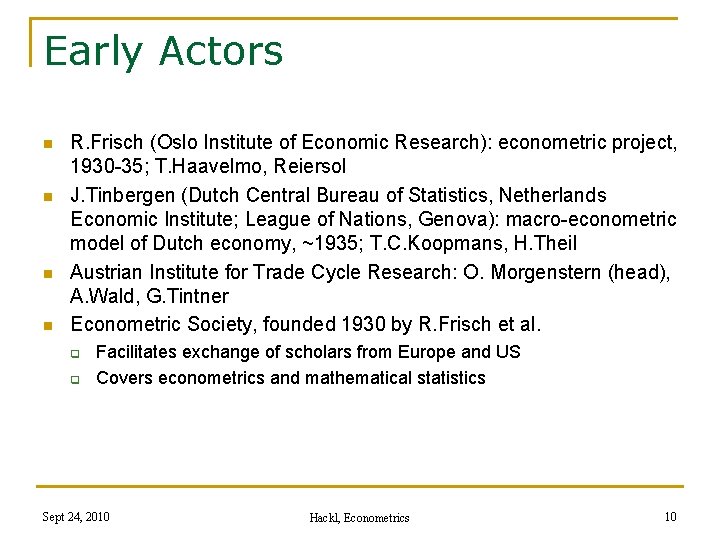
Early Actors n n R. Frisch (Oslo Institute of Economic Research): econometric project, 1930 -35; T. Haavelmo, Reiersol J. Tinbergen (Dutch Central Bureau of Statistics, Netherlands Economic Institute; League of Nations, Genova): macro-econometric model of Dutch economy, ~1935; T. C. Koopmans, H. Theil Austrian Institute for Trade Cycle Research: O. Morgenstern (head), A. Wald, G. Tintner Econometric Society, founded 1930 by R. Frisch et al. q q Facilitates exchange of scholars from Europe and US Covers econometrics and mathematical statistics Sept 24, 2010 Hackl, Econometrics 10

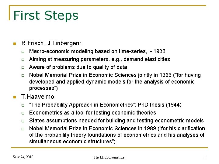
First Steps n R. Frisch, J. Tinbergen: q q n Macro-economic modeling based on time-series, ~ 1935 Aiming at measuring parameters, e. g. , demand elasticities Aware of problems due to quality of data Nobel Memorial Prize in Economic Sciences jointly in 1969 (“for having developed and applied dynamic models for the analysis of economic processes”) T. Haavelmo q q “The Probability Approach in Econometrics”: Ph. D thesis (1944) Econometrics as a tool for testing economic theories States assumptions needed for building and testing econometric models Nobel Memorial Prize in Economic Sciences in 1989 ("for his clarification of the probability theory foundations of econometrics and his analyses of simultaneous economic structures”) Sept 24, 2010 Hackl, Econometrics 11

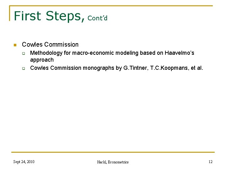
First Steps, Cont’d n Cowles Commission q q Methodology for macro-economic modeling based on Haavelmo’s approach Cowles Commission monographs by G. Tintner, T. C. Koopmans, et al. Sept 24, 2010 Hackl, Econometrics 12

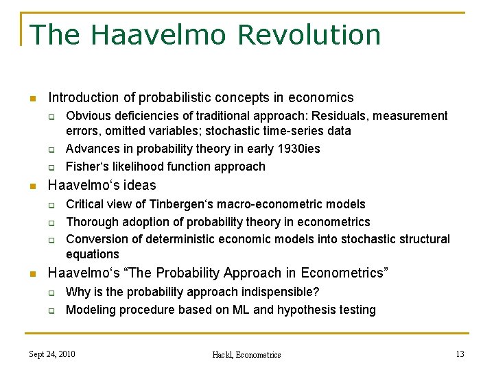
The Haavelmo Revolution n Introduction of probabilistic concepts in economics q q q n Haavelmo‘s ideas q q q n Obvious deficiencies of traditional approach: Residuals, measurement errors, omitted variables; stochastic time-series data Advances in probability theory in early 1930 ies Fisher‘s likelihood function approach Critical view of Tinbergen‘s macro-econometric models Thorough adoption of probability theory in econometrics Conversion of deterministic economic models into stochastic structural equations Haavelmo‘s “The Probability Approach in Econometrics” q q Why is the probability approach indispensible? Modeling procedure based on ML and hypothesis testing Sept 24, 2010 Hackl, Econometrics 13

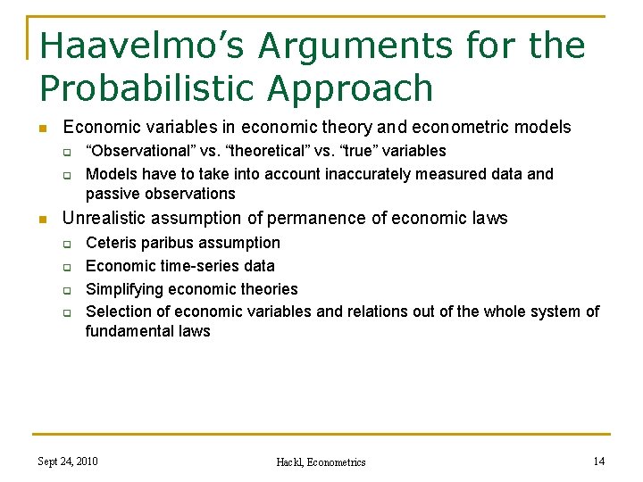
Haavelmo’s Arguments for the Probabilistic Approach n Economic variables in economic theory and econometric models q q n “Observational” vs. “theoretical” vs. “true” variables Models have to take into account inaccurately measured data and passive observations Unrealistic assumption of permanence of economic laws q q Ceteris paribus assumption Economic time-series data Simplifying economic theories Selection of economic variables and relations out of the whole system of fundamental laws Sept 24, 2010 Hackl, Econometrics 14

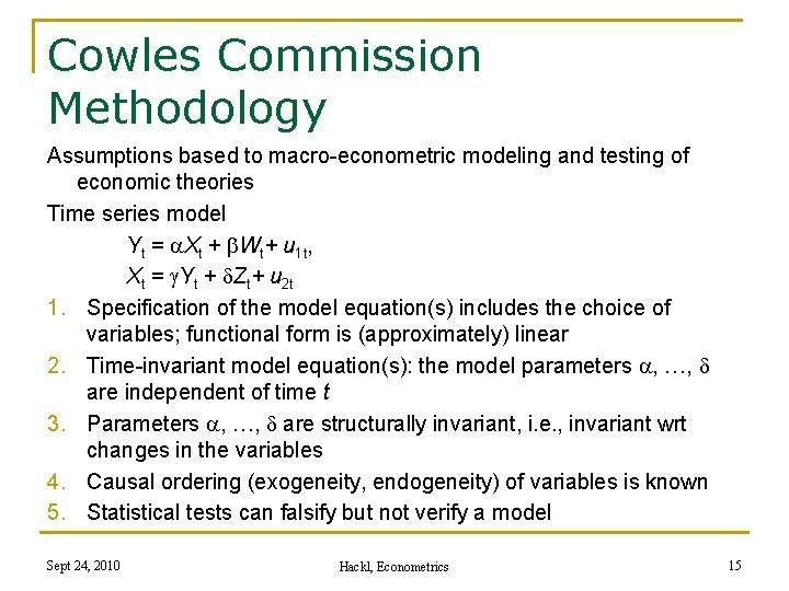
Cowles Commission Methodology Assumptions based to macro-econometric modeling and testing of economic theories Time series model Yt = a. Xt + Wt+ u 1 t, Xt = g. Yt + d. Zt+ u 2 t 1. Specification of the model equation(s) includes the choice of variables; functional form is (approximately) linear 2. Time-invariant model equation(s): the model parameters a, …, d are independent of time t 3. Parameters a, …, d are structurally invariant, i. e. , invariant wrt changes in the variables 4. Causal ordering (exogeneity, endogeneity) of variables is known 5. Statistical tests can falsify but not verify a model Sept 24, 2010 Hackl, Econometrics 15

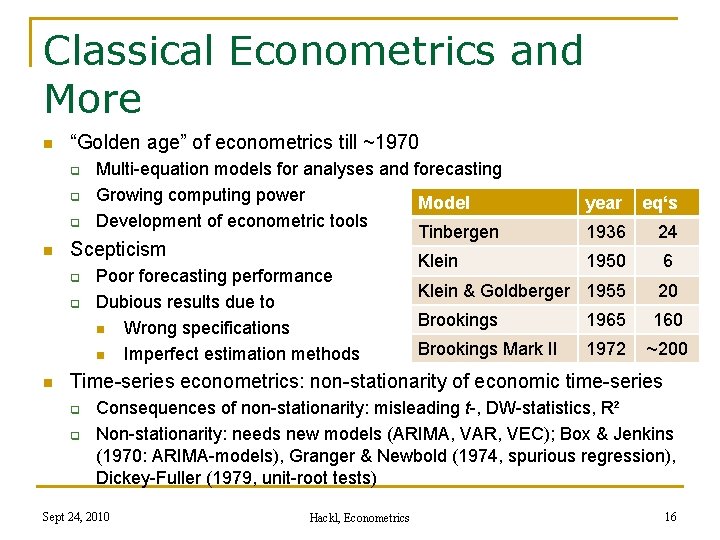
Classical Econometrics and More n “Golden age” of econometrics till ~1970 q q q n Scepticism q q n Multi-equation models for analyses and forecasting Growing computing power Model Development of econometric tools Tinbergen Poor forecasting performance Dubious results due to n Wrong specifications n Imperfect estimation methods year eq‘s 1936 24 1950 6 Klein & Goldberger 1955 20 Brookings 1965 160 Brookings Mark II 1972 ~200 Klein Time-series econometrics: non-stationarity of economic time-series q q Consequences of non-stationarity: misleading t-, DW-statistics, R² Non-stationarity: needs new models (ARIMA, VAR, VEC); Box & Jenkins (1970: ARIMA-models), Granger & Newbold (1974, spurious regression), Dickey-Fuller (1979, unit-root tests) Sept 24, 2010 Hackl, Econometrics 16

Econometrics … n n n … consists of the application of statistical data and techniques to mathematical formulations of economic theory. It serves to test the hypotheses of economic theory and to estimate the implied interrelationships. (Tinbergen, 1952) … is the interaction of economic theory, observed data and statistical methods. It is the interaction of these three that makes econometrics interesting, challenging, and, perhaps, difficult. (Verbeek, 2008) … is a methodological science with the elements q q Sept 24, 2010 economic theory mathematical language statistical methods software Hackl, Econometrics 17

The Course 1. Introduction to linear regression (Verbeek, Ch. 2): the linear regression model, OLS method, properties of OLS estimators 2. Introduction to linear regression (Verbeek, Ch. 2): goodness of fit, hypotheses testing, multicollinearity 3. Interpreting and comparing regression models (MV, Ch. 3): interpretation of the fitted model, selection of regressors, testing the functional form 4. Heteroskedascity and autocorrelation (Verbeek, Ch. 4): causes, consequences, testing, alternatives for inference 5. Endogeneity, instrumental variables and GMM (Verbeek, Ch. 5): the IV estimator, the generalized instrumental variables estimator, the generalized method of moments (GMM) 6. The practice of econometric modeling Sept 24, 2010 Hackl, Econometrics 18

The Next Course n n n Univariate and multivariate time series models: ARMA-, ARCH -, GARCH-models, VAR-, VEC-models Models for panel data Models with limited dependent variables: binary choice, count data Sept 24, 2010 Hackl, Econometrics 19

Contents n Organizational Issues Some History of Econometrics n An Introduction to Linear Regression n n q OLS as an algebraic tool q The Linear Regression Model q Small Sample Properties of OLS estimator Introduction to GRETL Sept 24, 2010 Hackl, Econometrics 20

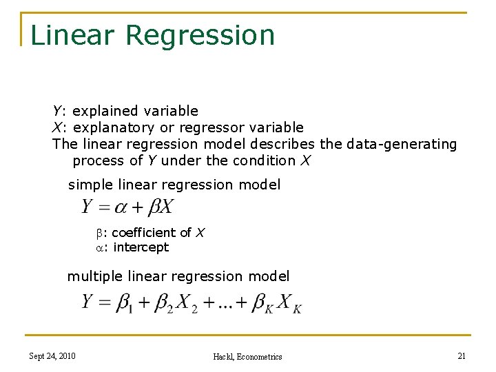
Linear Regression Y: explained variable X: explanatory or regressor variable The linear regression model describes the data-generating process of Y under the condition X simple linear regression model : coefficient of X a: intercept multiple linear regression model Sept 24, 2010 Hackl, Econometrics 21

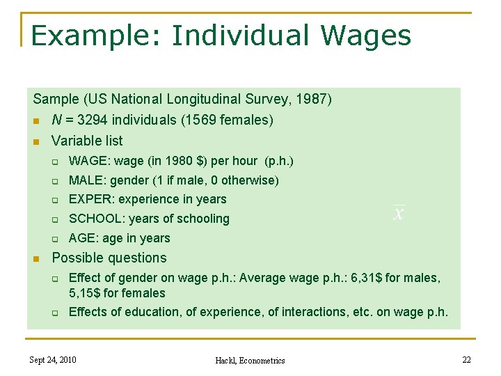
Example: Individual Wages Sample (US National Longitudinal Survey, 1987) n N = 3294 individuals (1569 females) n n Variable list q WAGE: wage (in 1980 $) per hour (p. h. ) q MALE: gender (1 if male, 0 otherwise) q EXPER: experience in years q SCHOOL: years of schooling q AGE: age in years Possible questions q q Effect of gender on wage p. h. : Average wage p. h. : 6, 31$ for males, 5, 15$ for females Effects of education, of experience, of interactions, etc. on wage p. h. Sept 24, 2010 Hackl, Econometrics 22

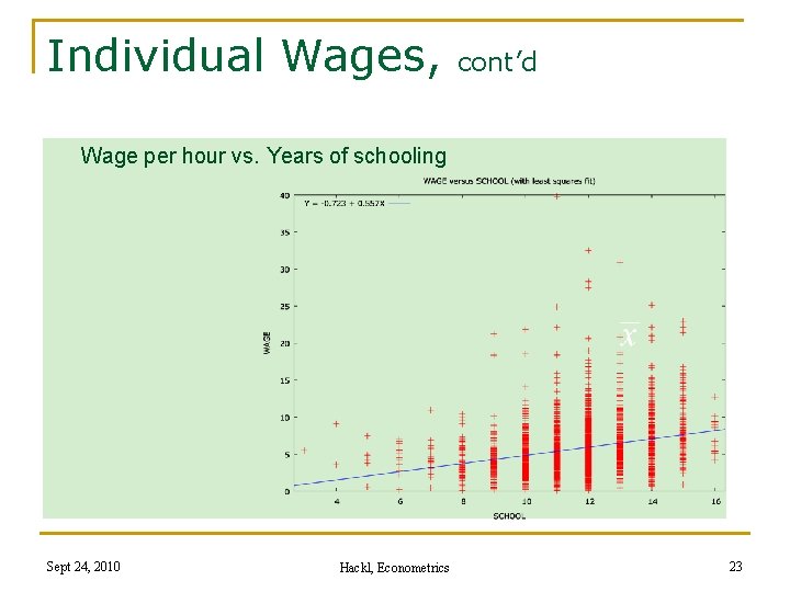
Individual Wages, cont’d Wage per hour vs. Years of schooling Sept 24, 2010 Hackl, Econometrics 23

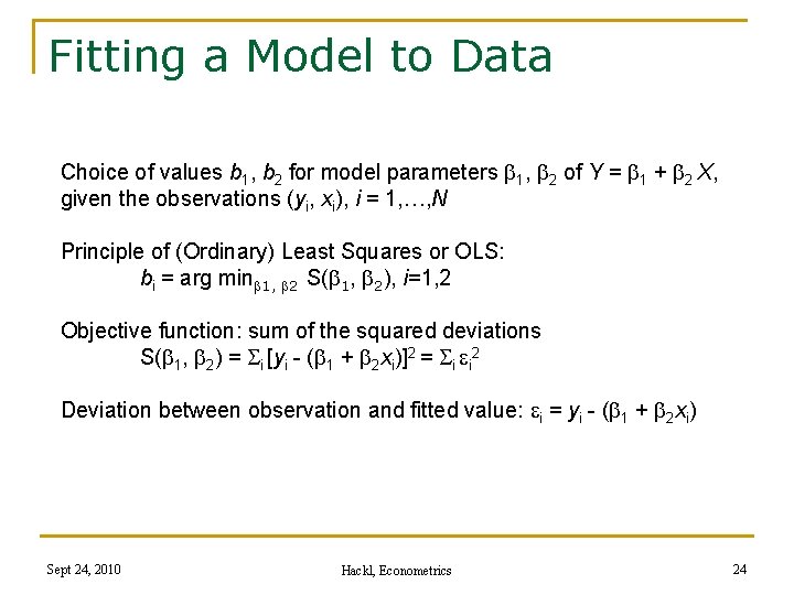
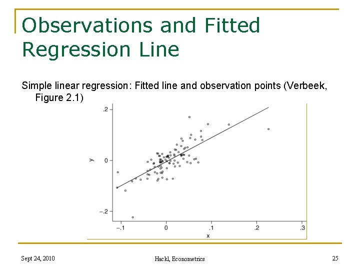
Fitting a Model to Data Choice of values b 1, b 2 for model parameters 1, 2 of Y = 1 + 2 X, given the observations (yi, xi), i = 1, …, N Principle of (Ordinary) Least Squares or OLS: bi = arg min 1, 2 S( 1, 2), i=1, 2 Objective function: sum of the squared deviations S( 1, 2) = Si [yi - ( 1 + 2 xi)]2 = Si i 2 Deviation between observation and fitted value: i = yi - ( 1 + 2 xi) Sept 24, 2010 Hackl, Econometrics 24

Observations and Fitted Regression Line Simple linear regression: Fitted line and observation points (Verbeek, Figure 2. 1) Sept 24, 2010 Hackl, Econometrics 25

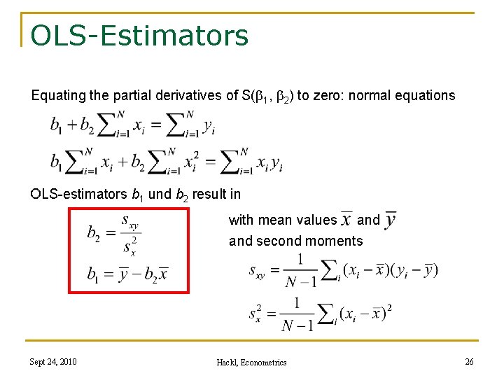
OLS-Estimators Equating the partial derivatives of S( 1, 2) to zero: normal equations OLS-estimators b 1 und b 2 result in with mean values and second moments Sept 24, 2010 Hackl, Econometrics 26

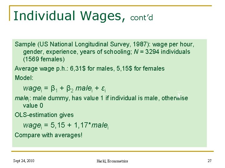
Individual Wages, cont’d Sample (US National Longitudinal Survey, 1987): wage per hour, gender, experience, years of schooling; N = 3294 individuals (1569 females) Average wage p. h. : 6, 31$ for males, 5, 15$ for females Model: wagei = β 1 + β 2 malei + εi male. I: male dummy, has value 1 if individual is male, otherwise value 0 OLS-estimation gives wagei = 5, 15 + 1, 17*malei Compare with averages! Sept 24, 2010 Hackl, Econometrics 27

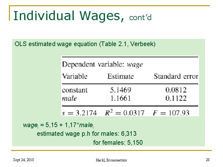
Individual Wages, cont’d OLS estimated wage equation (Table 2. 1, Verbeek) wagei = 5, 15 + 1, 17*malei estimated wage p. h for males: 6, 313 for females: 5, 150 Sept 24, 2010 Hackl, Econometrics 28

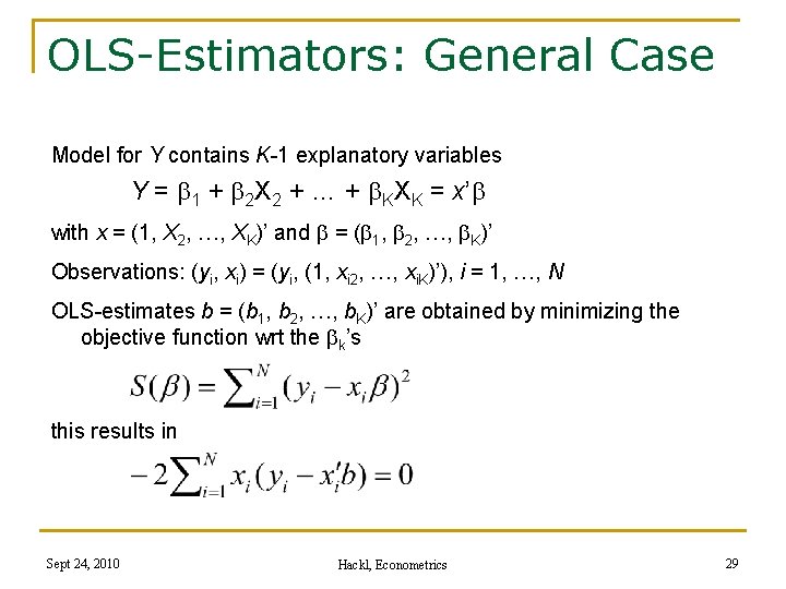
OLS-Estimators: General Case Model for Y contains K-1 explanatory variables Y = 1 + 2 X 2 + … + KXK = x’ with x = (1, X 2, …, XK)’ and = ( 1, 2, …, K)’ Observations: (yi, xi) = (yi, (1, xi 2, …, xi. K)’), i = 1, …, N OLS-estimates b = (b 1, b 2, …, b. K)’ are obtained by minimizing the objective function wrt the k’s this results in Sept 24, 2010 Hackl, Econometrics 29

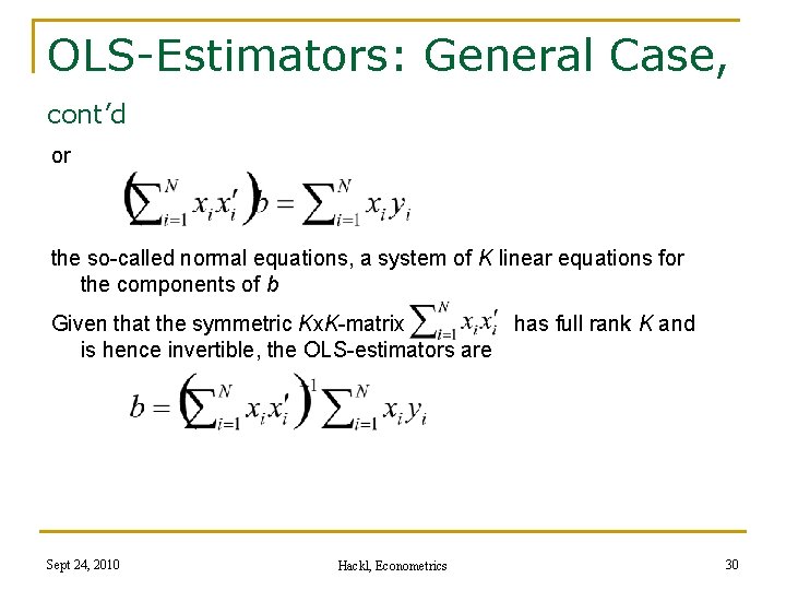
OLS-Estimators: General Case, cont’d or the so-called normal equations, a system of K linear equations for the components of b Given that the symmetric Kx. K-matrix has full rank K and is hence invertible, the OLS-estimators are Sept 24, 2010 Hackl, Econometrics 30

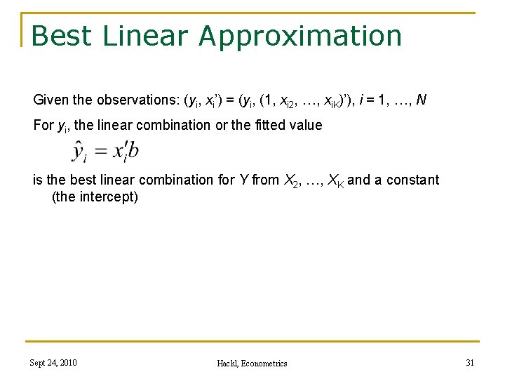
Best Linear Approximation Given the observations: (yi, xi’) = (yi, (1, xi 2, …, xi. K)’), i = 1, …, N For yi, the linear combination or the fitted value is the best linear combination for Y from X 2, …, XK and a constant (the intercept) Sept 24, 2010 Hackl, Econometrics 31

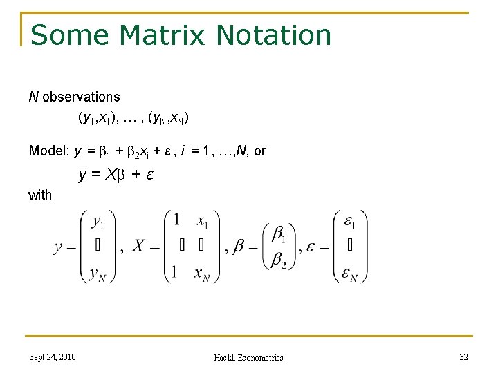
Some Matrix Notation N observations (y 1, x 1), … , (y. N, x. N) Model: yi = 1 + 2 xi + εi, i = 1, …, N, or y = X + ε with Sept 24, 2010 Hackl, Econometrics 32

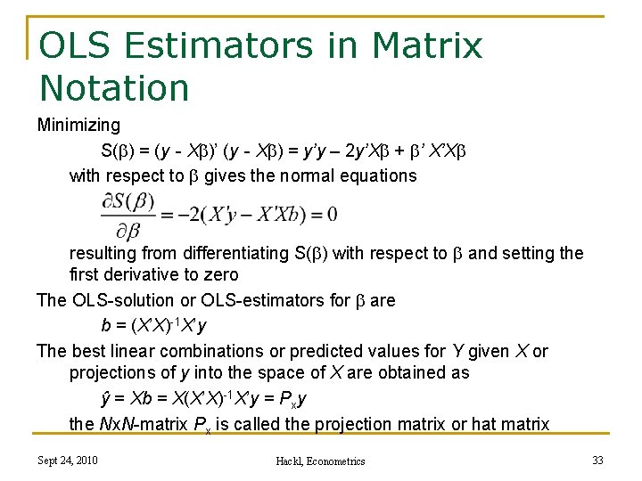
OLS Estimators in Matrix Notation Minimizing S( ) = (y - X )’ (y - X ) = y’y – 2 y’X + ’ X’X with respect to gives the normal equations resulting from differentiating S( ) with respect to and setting the first derivative to zero The OLS-solution or OLS-estimators for are b = (X’X)-1 X’y The best linear combinations or predicted values for Y given X or projections of y into the space of X are obtained as ŷ = Xb = X(X’X)-1 X’y = Pxy the Nx. N-matrix Px is called the projection matrix or hat matrix Sept 24, 2010 Hackl, Econometrics 33

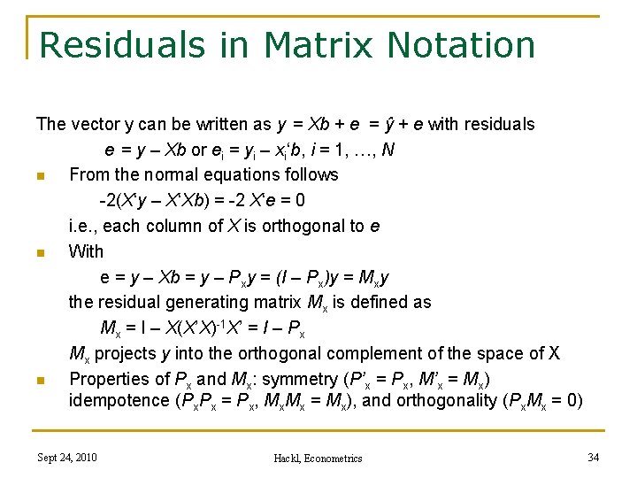
Residuals in Matrix Notation The vector y can be written as y = Xb + e = ŷ + e with residuals e = y – Xb or ei = yi – xi‘b, i = 1, …, N n From the normal equations follows -2(X‘y – X‘Xb) = -2 X‘e = 0 i. e. , each column of X is orthogonal to e n With e = y – Xb = y – Pxy = (I – Px)y = Mxy the residual generating matrix Mx is defined as Mx = I – X(X’X)-1 X’ = I – Px Mx projects y into the orthogonal complement of the space of X n Properties of Px and Mx: symmetry (P’x = Px, M’x = Mx) idempotence (Px. Px = Px, Mx. Mx = Mx), and orthogonality (Px. Mx = 0) Sept 24, 2010 Hackl, Econometrics 34

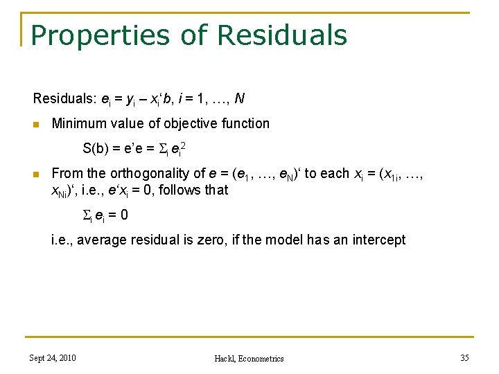
Properties of Residuals: ei = yi – xi‘b, i = 1, …, N n Minimum value of objective function S(b) = e’e = Si ei 2 n From the orthogonality of e = (e 1, …, e. N)‘ to each xi = (x 1 i, …, x. Ni)‘, i. e. , e‘xi = 0, follows that S i ei = 0 i. e. , average residual is zero, if the model has an intercept Sept 24, 2010 Hackl, Econometrics 35

Contents n Organizational Issues Some History of Econometrics n An Introduction to Linear Regression n n q OLS as an algebraic tool q The Linear Regression Model q Small Sample Properties of OLS estimator Introduction to GRETL Sept 24, 2010 Hackl, Econometrics 36

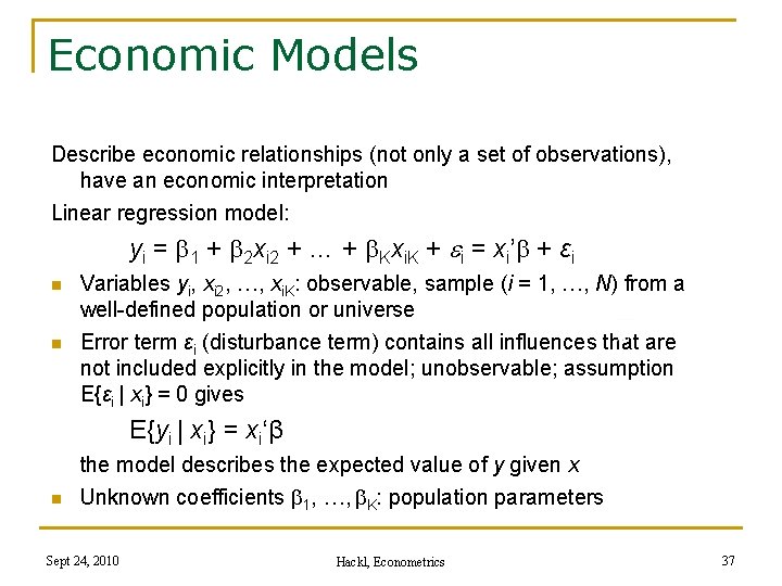
Economic Models Describe economic relationships (not only a set of observations), have an economic interpretation Linear regression model: yi = 1 + 2 xi 2 + … + Kxi. K + ei = xi’ + εi n n Variables yi, xi 2, …, xi. K: observable, sample (i = 1, …, N) from a well-defined population or universe Error term εi (disturbance term) contains all influences that are not included explicitly in the model; unobservable; assumption E{εi | xi} = 0 gives E{yi | xi} = xi‘β n the model describes the expected value of y given x Unknown coefficients 1, …, K: population parameters Sept 24, 2010 Hackl, Econometrics 37

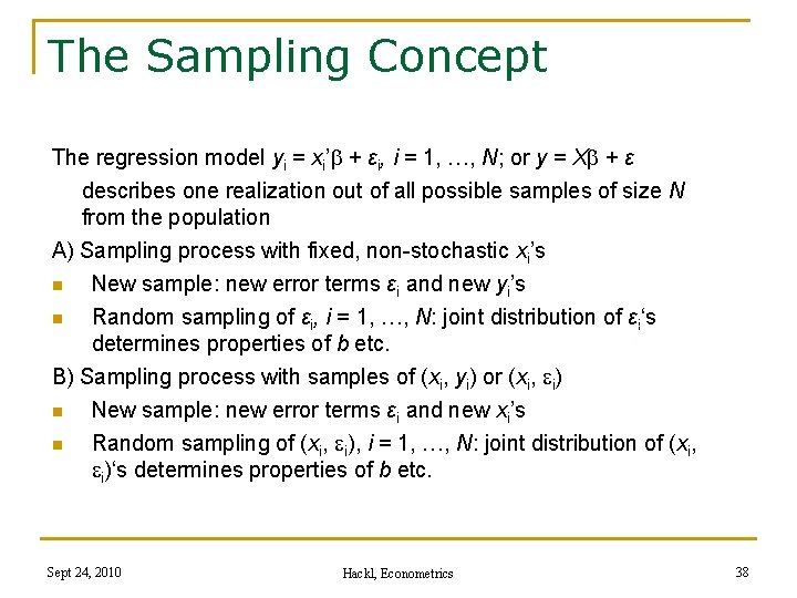
The Sampling Concept The regression model yi = xi’ + εi, i = 1, …, N; or y = X + ε describes one realization out of all possible samples of size N from the population A) Sampling process with fixed, non-stochastic xi’s n New sample: new error terms εi and new yi’s n Random sampling of εi, i = 1, …, N: joint distribution of εi‘s determines properties of b etc. B) Sampling process with samples of (xi, yi) or (xi, i) n New sample: new error terms εi and new xi’s n Random sampling of (xi, i), i = 1, …, N: joint distribution of (xi, i)‘s determines properties of b etc. Sept 24, 2010 Hackl, Econometrics 38

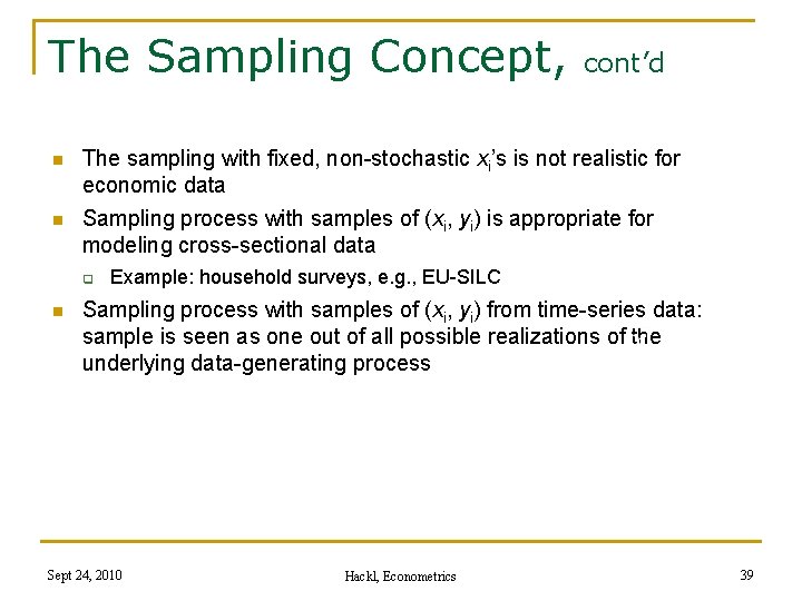
The Sampling Concept, cont’d n The sampling with fixed, non-stochastic xi’s is not realistic for economic data n Sampling process with samples of (xi, yi) is appropriate for modeling cross-sectional data q n Example: household surveys, e. g. , EU-SILC Sampling process with samples of (xi, yi) from time-series data: sample is seen as one out of all possible realizations of the underlying data-generating process Sept 24, 2010 Hackl, Econometrics 39

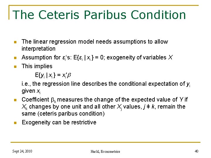
The Ceteris Paribus Condition n The linear regression model needs assumptions to allow interpretation n Assumption for εi‘s: E{εi | xi } = 0; exogeneity of variables X This implies E{yi | xi } = xi'b i. e. , the regression line describes the conditional expectation of yi given xi Coefficient k measures the change of the expected value of Y if Xk changes by one unit and all other Xj values, j ǂ k, remain the same (ceteris paribus condition) Exogeneity can be restrictive n n n Sept 24, 2010 Hackl, Econometrics 40

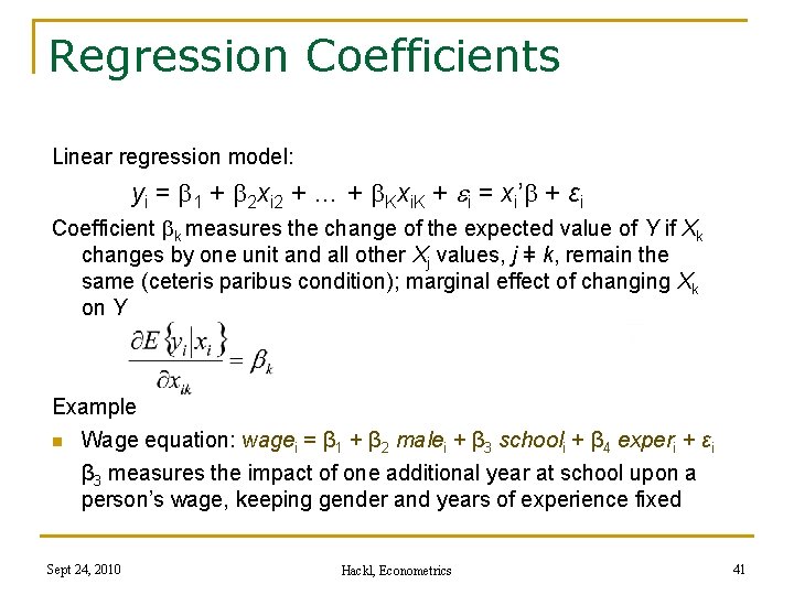
Regression Coefficients Linear regression model: yi = 1 + 2 xi 2 + … + Kxi. K + ei = xi’ + εi Coefficient k measures the change of the expected value of Y if Xk changes by one unit and all other Xj values, j ǂ k, remain the same (ceteris paribus condition); marginal effect of changing Xk on Y Example n Wage equation: wagei = β 1 + β 2 malei + β 3 schooli + β 4 experi + εi β 3 measures the impact of one additional year at school upon a person’s wage, keeping gender and years of experience fixed Sept 24, 2010 Hackl, Econometrics 41

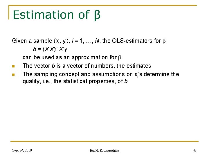
Estimation of β Given a sample (xi, yi), i = 1, …, N, the OLS-estimators for b = (X’X)-1 X’y can be used as an approximation for n The vector b is a vector of numbers, the estimates n The sampling concept and assumptions on εi‘s determine the quality, i. e. , the statistical properties, of b Sept 24, 2010 Hackl, Econometrics 42

Contents n Organizational Issues Some History of Econometrics n An Introduction to Linear Regression n n q OLS as an algebraic tool q The Linear Regression Model q Small Sample Properties of OLS estimator Introduction to GRETL Sept 24, 2010 Hackl, Econometrics 43

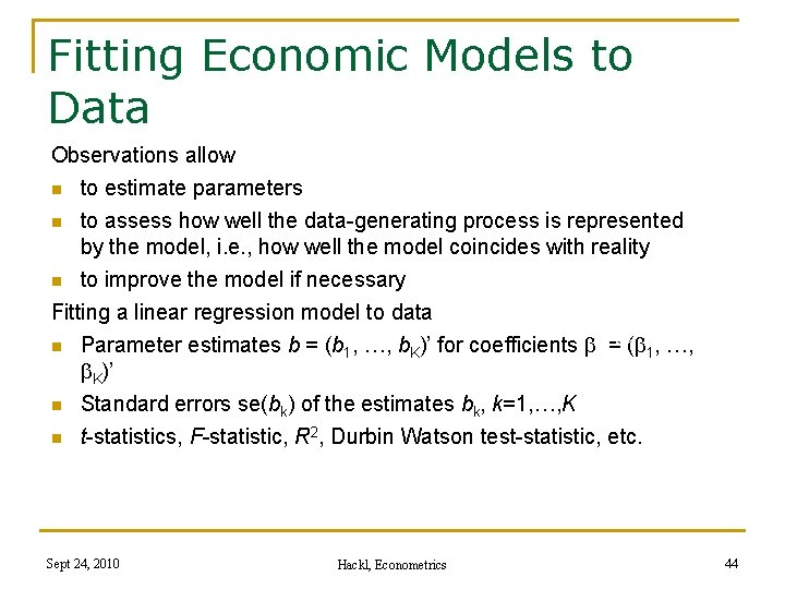
Fitting Economic Models to Data Observations allow n to estimate parameters to assess how well the data-generating process is represented by the model, i. e. , how well the model coincides with reality n to improve the model if necessary Fitting a linear regression model to data n Parameter estimates b = (b 1, …, b. K)’ for coefficients = ( 1, …, K)’ n Standard errors se(bk) of the estimates bk, k=1, …, K n t-statistics, F-statistic, R 2, Durbin Watson test-statistic, etc. n Sept 24, 2010 Hackl, Econometrics 44

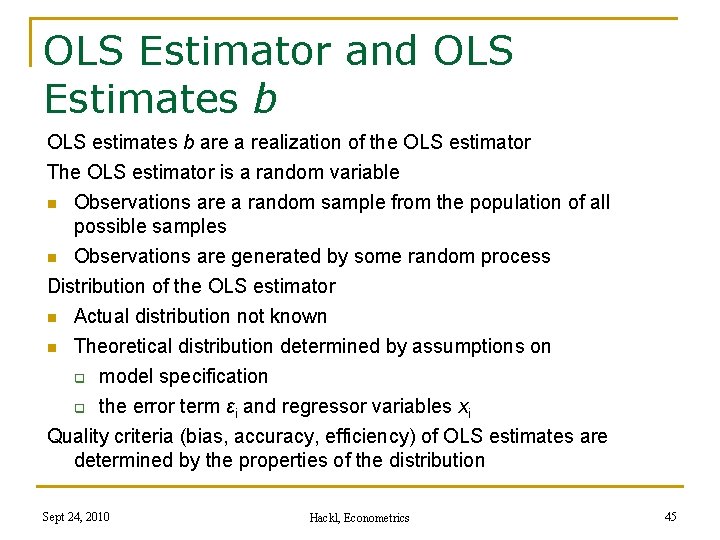
OLS Estimator and OLS Estimates b OLS estimates b are a realization of the OLS estimator The OLS estimator is a random variable Observations are a random sample from the population of all possible samples n Observations are generated by some random process Distribution of the OLS estimator n Actual distribution not known n Theoretical distribution determined by assumptions on q model specification q the error term εi and regressor variables xi Quality criteria (bias, accuracy, efficiency) of OLS estimates are determined by the properties of the distribution n Sept 24, 2010 Hackl, Econometrics 45

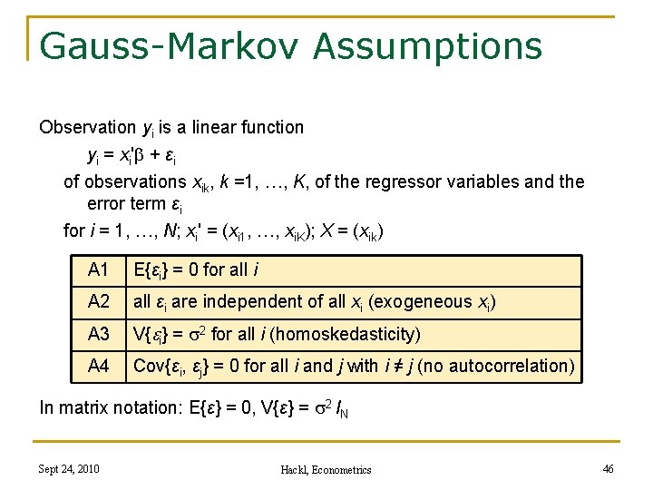
Gauss-Markov Assumptions Observation yi is a linear function yi = xi' + εi of observations xik, k =1, …, K, of the regressor variables and the error term εi for i = 1, …, N; xi' = (xi 1, …, xi. K); X = (xik) A 1 E{εi} = 0 for all i A 2 all εi are independent of all xi (exogeneous xi) A 3 V{ei} = s 2 for all i (homoskedasticity) A 4 Cov{εi, εj} = 0 for all i and j with i ≠ j (no autocorrelation) In matrix notation: E{ε} = 0, V{ε} = s 2 IN Sept 24, 2010 Hackl, Econometrics 46

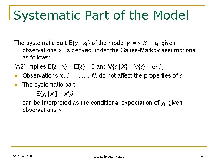
Systematic Part of the Model The systematic part E{yi | xi } of the model yi = xi'b + εi, given observations xi, is derived under the Gauss-Markov assumptions as follows: (A 2) implies E{ε | X} = E{ε} = 0 and V{ε | X} = V{ε} = s 2 IN n Observations xi, i = 1, …, N, do not affect the properties of ε n The systematic part E{yi | xi } = xi'b can be interpreted as the conditional expectation of yi, given observations xi Sept 24, 2010 Hackl, Econometrics 47

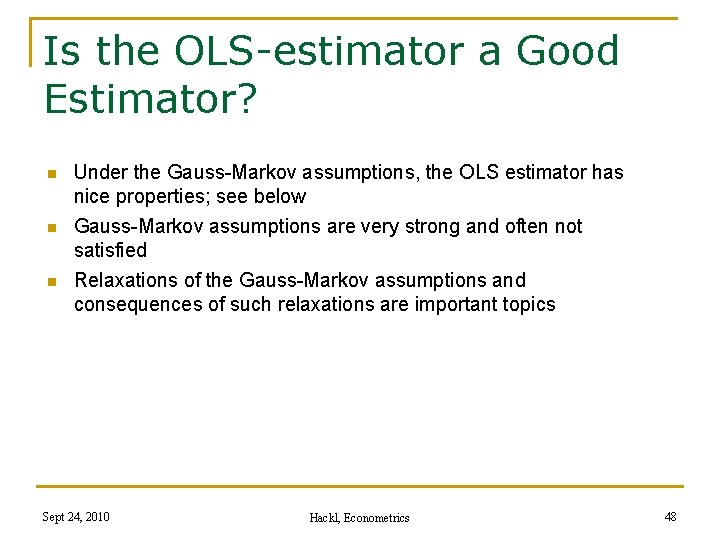
Is the OLS-estimator a Good Estimator? n n n Under the Gauss-Markov assumptions, the OLS estimator has nice properties; see below Gauss-Markov assumptions are very strong and often not satisfied Relaxations of the Gauss-Markov assumptions and consequences of such relaxations are important topics Sept 24, 2010 Hackl, Econometrics 48

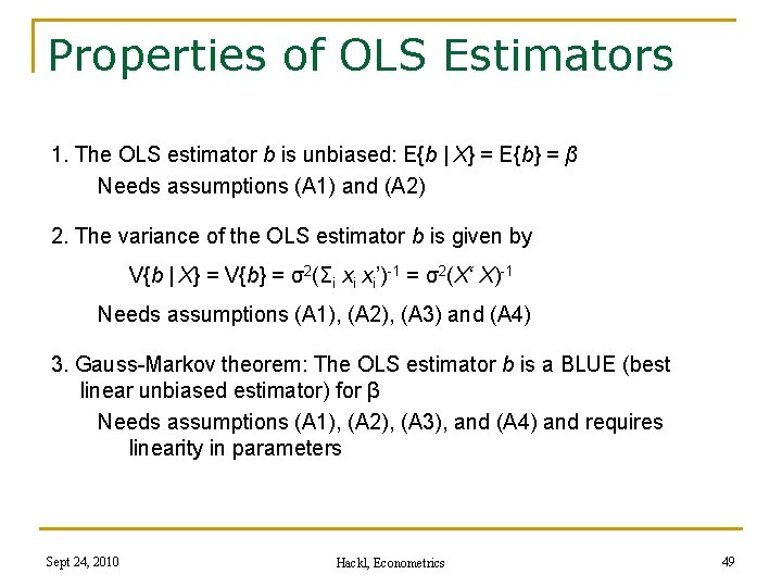
Properties of OLS Estimators 1. The OLS estimator b is unbiased: E{b | X} = E{b} = β Needs assumptions (A 1) and (A 2) 2. The variance of the OLS estimator b is given by V{b | X} = V{b} = σ2(Σi xi xi’)-1 = σ2(X‘ X)-1 Needs assumptions (A 1), (A 2), (A 3) and (A 4) 3. Gauss-Markov theorem: The OLS estimator b is a BLUE (best linear unbiased estimator) for β Needs assumptions (A 1), (A 2), (A 3), and (A 4) and requires linearity in parameters Sept 24, 2010 Hackl, Econometrics 49

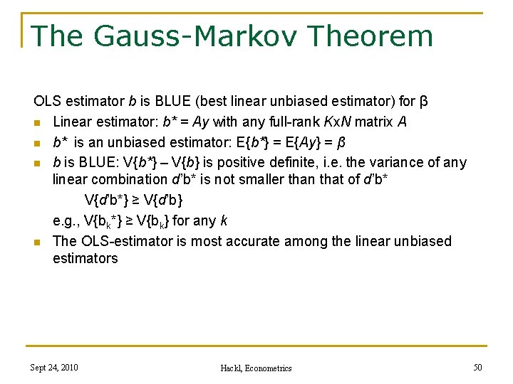
The Gauss-Markov Theorem OLS estimator b is BLUE (best linear unbiased estimator) for β n Linear estimator: b* = Ay with any full-rank Kx. N matrix A n b* is an unbiased estimator: E{b*} = E{Ay} = β n b is BLUE: V{b*} – V{b} is positive definite, i. e. the variance of any linear combination d’b* is not smaller than that of d’b* V{d’b*} ≥ V{d’b} e. g. , V{bk*} ≥ V{bk} for any k n The OLS-estimator is most accurate among the linear unbiased estimators Sept 24, 2010 Hackl, Econometrics 50

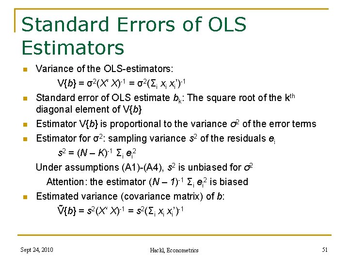
Standard Errors of OLS Estimators n Variance of the OLS-estimators: V{b} = σ2(X‘ X)-1 = σ2(Σi xi xi’)-1 n Standard error of OLS estimate bk: The square root of the kth diagonal element of V{b} Estimator V{b} is proportional to the variance σ2 of the error terms Estimator for σ2: sampling variance s 2 of the residuals ei s 2 = (N – K)-1 Σi ei 2 Under assumptions (A 1)-(A 4), s 2 is unbiased for σ2 Attention: the estimator (N – 1)-1 Σi ei 2 is biased Estimated variance (covariance matrix) of b: Ṽ{b} = s 2(X‘ X)-1 = s 2(Σi xi xi’)-1 n n n Sept 24, 2010 Hackl, Econometrics 51

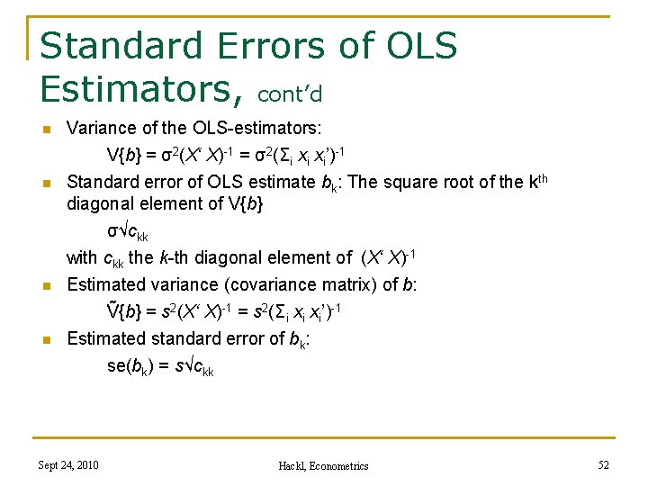
Standard Errors of OLS Estimators, cont’d n Variance of the OLS-estimators: V{b} = σ2(X‘ X)-1 = σ2(Σi xi xi’)-1 n Standard error of OLS estimate bk: The square root of the kth diagonal element of V{b} σ√ckk with ckk the k-th diagonal element of (X‘ X)-1 Estimated variance (covariance matrix) of b: Ṽ{b} = s 2(X‘ X)-1 = s 2(Σi xi xi’)-1 Estimated standard error of bk: se(bk) = s√ckk n n Sept 24, 2010 Hackl, Econometrics 52

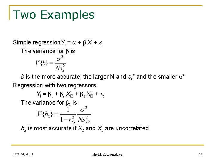
Two Examples Simple regression. Yi = a + Xi + et The variance for is b is the more accurate, the larger N and sx² and the smaller s² Regression with two regressors: Yi = 1 + 2 Xi 2 + 3 Xi 3 + et The variance for 2 is b 2 is most accurate if X 2 and X 3 are uncorrelated Sept 24, 2010 Hackl, Econometrics 53

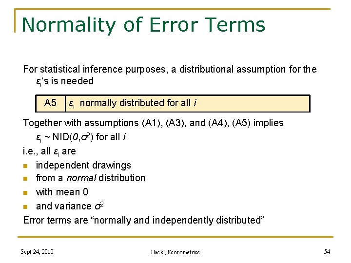
Normality of Error Terms For statistical inference purposes, a distributional assumption for the εi‘s is needed A 5 εi normally distributed for all i Together with assumptions (A 1), (A 3), and (A 4), (A 5) implies εi ~ NID(0, σ2) for all i i. e. , all εi are n independent drawings n from a normal distribution n with mean 0 n and variance σ2 Error terms are “normally and independently distributed” Sept 24, 2010 Hackl, Econometrics 54

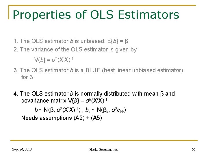
Properties of OLS Estimators 1. The OLS estimator b is unbiased: E{b} = β 2. The variance of the OLS estimator is given by V{b} = σ2(X’X)-1 3. The OLS estimator b is a BLUE (best linear unbiased estimator) for β 4. The OLS estimator b is normally distributed with mean β and covariance matrix V{b} = σ2(X‘X)-1 b ~ N(β, σ2(X’X)-1) , bk ~ N(βk, σ2 ckk) Needs assumptions (A 2) + (A 5) Sept 24, 2010 Hackl, Econometrics 55

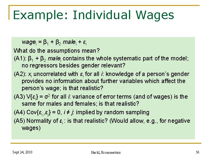
Example: Individual Wages wagei = β 1 + β 2 malei + εi What do the assumptions mean? (A 1): β 1 + β 2 malei contains the whole systematic part of the model; no regressors besides gender relevant? (A 2): xi uncorrelated with εi for all i: knowledge of a person’s gender provides no information about further variables which affect the person’s wage; is that realistic? (A 3) V{εi} = σ2 for all i: variance of error terms (and of wages) is the same for males and females; is that realistic? (A 4) Cov{εi, , εj} = 0, i ≠ j: implied by random sampling (A 5) Normality of εi : is that realistic? (Would allow, e. g. , for negative wages) Sept 24, 2010 Hackl, Econometrics 56

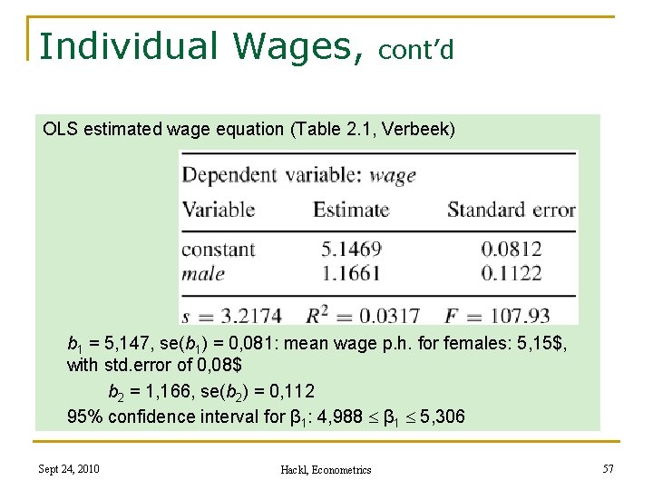
Individual Wages, cont’d OLS estimated wage equation (Table 2. 1, Verbeek) b 1 = 5, 147, se(b 1) = 0, 081: mean wage p. h. for females: 5, 15$, with std. error of 0, 08$ b 2 = 1, 166, se(b 2) = 0, 112 95% confidence interval for β 1: 4, 988 β 1 5, 306 Sept 24, 2010 Hackl, Econometrics 57

Your Homework 1. Verbeek’s data set “WAGES” contains for a sample of 3294 individuals the wage and other variables. Using GRETL, draw box plots (a) for all wages p. h. in the sample, (b) for wages p. h. of males and of females. 2. For Verbeek’s data set “WAGES”, calculate, using GRETL, the mean wage p. h. (a) of the whole sample, (b) of males and females, and (c) of persons with schooling between (i) 0 and 6 years, (ii) 7 and 12 years, and (iii) 13 and 16 years. 3. For the simple linear regression (Y = 1 + 2 X + ): write the OLS -estimator b = (X’X)-1 X’y in summation form; X: Nx. K. 4. Show that V{b} = σ2(X‘X)-1. 5. Show that Px. Mx = 0 for the hat matrix Px and the residual generating matrix Mx. Sept 24, 2010 Hackl, Econometrics 58