Econometrics for managers Debre Markos university 2020 INTRODUCTION

Econometrics for managers Debre Markos university 2020

INTRODUCTION: The Basics of Econometrics • Econometrics means “economic measurement”. The scope of econometrics is much broader, as can be seen from the following definitions: 1. “Consists of the application of mathematical statistics to economic data to lend empirical support to the models constructed by mathematical economics and to obtain numerical results” (Gerhard, 1968). 2. “Econometrics may be defined as the social science in which the tools of economic theory, mathematics, and statistical inference are applied to the analysis of economic phenomena” (Goldberger, 1964). 3. “Econometrics is concerned with the empirical determination of economic laws” (Theil, 1971). 4. Econometrics is the quantitative analysis of actual economic phenomena based on concurrent development of theory and observation, related by appropriate methods of inference (Samuelsonet al. , 1954).

Con’d The subject of Econometrics deserves to be studied in its own right for the following reasons: 1. Economic theory makes statements or hypotheses that are mostly qualitative in nature (the law of demand), the law does not provide any numerical measure of the relationship. This is the job of the econometrician. 2. The main concern of mathematical economics is to express economic theory in mathematical form without regard to measurability or empirical verification of theory. Econometrics is mainly interested in the empirical verification of economic theory. 3. Economic statistics is mainly concerned with collecting, processing, and presenting economic data in the form of charts and tables. It does not go any further. The one who does that is the econometrician. 4. Mathematical statistics provides many of the tools for economic studies, but econometrics supplies the later with many special methods of quantitative analysis based on economic data.

Methodology of econometrics • Broadly speaking, traditional econometric methodology proceeds along the following lines: – – – – Statement of theory or hypothesis, Specification of the mathematical model of theory, Specification of the statistical, or econometric, model, Collecting the data, Estimation of the parameters of the econometric model, Hypothesis testing, Forecasting or prediction, and Using the model for control or policy purposes.


Linear Correlation Analysis ü The presence of linear correlation between two random variables can be detected by linear correlation analysis. The covariance of two random variables, x and y, can be expressed as ü The relationship between x and y may be of three types: a. Cov(x, y) > 0 positive correlation b. Cov(x, y) <0 negative correlation c. Cov(x, y) =0 independent

Con’d • The correlation coefficient measures the relative strength of the linear relationship between two variables, which is unit-less. It ranges between – 1 and 1. The closer to – 1, the stronger the negative linear relationship, the closer to 1, the stronger the positive linear relationship, and the closer to 0, the weaker is any positive linear relationship. The Pearson’s correlation coefficient is the standardized covariance:

Scatter plots of data with various correlation coefficients

Illustration of linear and nonlinear relationships

Con’d • In correlation, the two variables are treated as equals. • In regression, one variable is considered independent (or predictor) variable (x) and the other the dependent (or outcome) variable y. • If you know something about x, this knowledge helps us predict something about y (sound like conditional probabilities).

Con’d • Econometrics is different from correlation as Econometrics is the application of statistical, and mathematical techniques to the analysis of economic data with a purpose of verifying or refuting economic theories.

Significance of the Stochastic Disturbance Term ü The disturbance term is a surrogate for all those variables that are omitted from the model but that collectively affect y. The obvious question is: Why not introduce these variables into the model explicitly? Stated otherwise, why not develop a multiple regression model with as many variables as possible? The reasons are many. Ø Vagueness of theory: The theory, if any, determining the behavior of y may be, and often is, incomplete. Ø Unavailability of data. Ø Core variables vs. peripheral variables: It is quite possible that the joint influence of all or some of the variables may be so small and at best nonsystematic or random that as a practical matter and for cost considerations it does not pay to introduce them into the model explicitly. One hopes that their combined effect can be treated as a random variable.

Con’d Ø Intrinsic randomness in human behavior: Even if we succeed in introducing all the relevant variables into the model, there is bound to be some “intrinsic” randomness in individual y' s that cannot be explained no matter how hard we try. The disturbances may very well reflect this intrinsic randomness. Ø Poor proxy variables: Although the classical regression model assumes that the variables yand xare measured accurately, in practice the data may be plagued by errors of measurement. Ø Principle of parsimony: Following Occam’s razor, we would like to keep our regression model as simple as possible. If we can explain the behavior of y“substantially” with two or three explanatory variables and if our theory is not strong enough to suggest what other variables might be included, why introduce more variables? Let the disturbance termrepresent all other variables. Of course, we should not exclude relevant and important variables just to keep the regression model simple. Ø Wrong functional form: Even if we have theoretically correct variables explaining a phenomenon and even if we can obtain data on these variables, very often we do not know the form of the functional relationship between the regressand the regressors.

Scale of measurements • Nominal Scale: Consists of ‘naming’ observations or classifying them into various mutually exclusive categories. • classified by some quality it possesses rather than by an amount or quantity. example: Religion: Christianity, Islam, Hinduism, etc. ; Sex: Male, Female • Ordinal Scale: Whenever observations are not only different from category to category, but can be ranked according to some criterion. The variables deal with their relative difference rather than with quantitative differences. • have meaningful inequalities. Example: Individuals may be classified according to socio-economic as low, medium & high

Con’d • Interval Scale: not only possible to order measurements, but also the distance between any two measurements is known but not meaningful quotients. Example: time period in years like 1989, 2015 etc • Ratio Scale: - continues variable : Example: Variables such as age, height, length, income, etc Types of data (variables) a. Time series: a set of observations on the values that a variable takes at different times. b. Cross-sectional data: data on one or more variables collected at the same point in time c. Pooled data: combination of time series and cross-section data d. Panel data: a special type of pooled data in which the same cross-section unit is surveyed overtime.

Variables can be classified as continuous and discrete variables. • Continuous Variables: - are usually obtained by measurement not by counting. These are variables which assume or take any decimal value when collected. The variables like age, time, height, income, price, temperature, and etc are all continuous since the data collected from such variables can take decimal values. • Discrete Variables: - are obtained by counting. A discrete variable takes always whole number values that are counted. Example variables such as number of students, number of errors per page, number of accidents on traffic line, number of defective or non-defective items produced in production line. Various econometricians used different ways of wordings to define econometrics. But if we distill the fundamental features/concepts of all the definitions, we may obtain the following definition.

Definition of the Simple Regression Model • premise: y and x are two variables, representing some population, and we are interested in “explaining y in terms of x, ” or in “studying how y varies with changes in x. ” • example: y is hourly wage and x is years of education • In writing down a model that will “explain y in terms of x, ” we must confront three issues. A. there is never an exact relationship between two variables, how do we allow for other factors to affect y? B. what is the functional relationship between y and x? C. how can we be sure we are capturing a ceteris paribus relationship between y and x? We can resolve these ambiguities by writing down an equation relating y to x. A simple equation is ……. (1)
defines the simple linear regression model. It is also called the")
• Equation (1)defines the simple linear regression model. It is also called the two-variable linear regression model or bivariate linear regression model because it relates the two variables x and y.
 model A 1: Linear in parameters:")
The basic assumption of multiple linear regression (MLR) model A 1: Linear in parameters: • The regression model is linear in the parameters (between y and x): A 2: Random sampling: • Random sampling of n observations: (xi , yi ): i = 1, 2, . . . , n. A 3: Sample variation: • There must be sufficient variability in the values taken by the regressors, xi’s are not all the same value: A 4: Zero conditional mean: • The error has an expected value of 0, given any values of the explanatory variable: E(e/ x) = 0.

Con’d A 5: Homoscedasticity: • The error has the same variance given any value of the explanatory variable: Var(e/ x) = s 2. For given x' s , the variance of e i is constant or homoscedastic. A 6: x values are fixed in repeated sampling: x is assumed to be nonstochastic A 7: No autocorrelation between the disturbances. A 8: Exogeneity of the independent variables: A 9: The number of observations n must be greater than the number of parameters to be estimated. A 10: No specification error: • The regression model is correctly specified. • A 11: No perfect collinearity: That is, there are no perfect linearrelationships among the explanatory variables.
 • Graphic decomposition of effects")
Deriving ordinary least squares (OLS) • Graphic decomposition of effects

Con’d Given a simple linear regression model: • Depending on the nature of data and functional form there are different techniques of estimating parameters in which OLS one of most widely used technique.

Con’d

Con’d

Statistical Properties of OLS Estimators • Given the assumptions of the classical linear regression model, the OLS estimates possess some ideal or optimum properties. These properties are contained in the well-known Gauss – Markov theorem. • I. An estimator is said to be a (BLUE) estimator if : It is linear, that is, a linear function of a random variable, such as the dependent variable y in the regression model. II. It is unbiased, that is, its average or expected value is equal to the true value. III. It has minimum variance in the class of all such linear unbiased estimators; an unbiased estimator with the least variance is known as an efficient estimator.

Con’d • Gauss–Markov theorem: Given the assumptions of the classical linear regression model, the least-squares estimators, in the class of unbiased linear estimators, have minimum variance, that is, they are BLUE. a. Linearity in parameters • The linearity assumption is a key to understanding of OLS models. The restriction is that our model of the population must be linear in the parameters:

Con’d • OLS model cannot be non-linear in the parameters. Non-linear in the variables (x's) , however, is fine and quite useful:

Con’d B. Unbiasedness • Average or expected value of the estimator equals true value of the population parameter. • The implication is that sampling distribution of the parameters is centered around the population parameter and hence they are unbiased estimator of the population parameters.

Demonstration of unbiasedness and efficiency of estimators with normal distribution

Con’d c. Efficiency • An estimator is efficient if it is unbiased and no other unbiased estimator has a smaller variance i. e. it has the minimum possible variance. • OLS estimators are the Best Linear Unbiased Estimators of the population parameters when the first 5 assumptions of the linear model, the Gauss-Markov theorem, hold: linear, unbiased, and efficient (have smaller variance than any other linear unbiased estimator). We might want to choose a biased estimator, if it has a smaller variance. They fulfill the five Gauss-Markov (G-M) assumptions: a. OLS estimators are the “best” among all linear and unbiased estimators. b. They are efficient: i. e. they have smallest variance among all other linear and unbiased estimators

Con’d c. Normality is unnecessary to assume; G-M result does not depend on normality of dependent variable. d. Gauss-Markov theorem refers to the estimators not to actual values of sample estimates calculated from a particular sample. e. Gauss-Markov theorem applies only to linear and unbiased estimators, there are other types of estimators which we can use and these may be better in which case disregard the Gauss-Markov theorem: e. g. a biased estimator may be more efficient than an unbiased one which fulfills this theorem.

Con’d d. Consistency • Other properties hold for “small” samples: Consistency is a large sample property i. e. asymptotic property. As n ®¥, the sampling distribution of the estimators collapses to the population parameters. This holds if the variance of the estimators approaches zero as the sample size approaches infinity. True estimators of the parameters are consistent estimators. The population variance, s 2, is an unknown population parameter: variance of the unobservable error terms:

• If the bias and variance both decrease as n gets larger, the estimator is consistent. Asymptotic efficiency requires asymptotic distribution with finite mean and variance, is consistent, and no estimator has smaller asymptotic variance. • Demonstration of consistency

Goodness of Fit • Coefficient of determination is a measure in a simple linear regression analysis that shows the explanatory power of independent variables (regressors) in explaining the variation on dependent variable (regressand). The total variation on the dependent variable can be decomposed as follows: • For n observations and k explanatory variables, the total variation in the dependent variable can be decomposed into explained and unexplained variation.

Con’d

Con’d • R 2 is the ratio of the explained variation compared to the total variation, or the fraction of the sample variation in y that is explained by x. R 2 always lies between zero and 1. If R 2=1, all actual points lie on the regression line (usually an error). If R 2≈0, the regression explains very little; OLS is a “poor fit”. The coefficient of determination is explained in a number of ways: 1. R 2 is defined in terms of variation about the mean of y so that if a model is re- parameterised (rearranged) and the dependent variable changes, R 2 will change. 2. R 2 never falls if more regressors are added to the regression. 3. R 2 quite often takes on values of 0. 9 or higher for time series regressions. In order to get around these problems, a modification is often made which takes into account the loss of degrees of freedom associated with adding extra variables. This is known as adjusted R 2. So if we add an extra regressor, k increases and unless R 2 increases by a more than offsetting amount, will actually fall. There are still problems with the criterion because there is no distribution for R 2.

Con’d

Residual Analysis • We need to check the many assumptions of regression about the errors by examining the residuals I. Examine for linearity assumption (Figure 8 a), II. Examine for constant variance for all levels of x of homoscedasticity (Figure 8 b), III. Evaluate normal distribution assumption, and IV. Evaluate independence assumption.

Graphical analysis of residuals for linearity and homoscedasticity assumptions

The test for normality assumption: • In general we assume the error term is normally distributed. The normality of the error term can be tested using the Jarque-Bera test, which tests for the presence of skewness (non-symmetry) and kurtosis (fat tails). This test for normality in effect tests for the coefficients of skewness and excess kurtosis being jointly equal to 0; • where S =coefficient of skewness, K = coefficient of excess kurtosis of residuals, and n =number of observations.

Con’d Ø For a normally distributed variable, S = 0 and K = 3. Ø Therefore, the JB test of normality is a test of the joint hypothesis that S and K are 0 and 3, respectively. Ø In that case the value of the JB statistic is expected to be 0. Ø Under the null hypothesis that the residuals are normally distributed, Jarque and Bera showed that asymptotically (i. e. , in large samples) the JB statistic follows the chi-square distribution with 2 df. Ø If the computed p value of the JB statistic in an application is sufficiently low, which will happen if the value of the statistic is very different from 0, one can reject the hypothesis that the residuals are normally distributed. But if the p value is reasonably high, which will happen if the value of the statistic is close to zero, we do not reject the normality assumption.
")
Analysis of residuals for independence (or exogeneity)

Basics of Hypothesis Testing • Even if the estimators are right on average, we still want to know how far off they might be in a given sample. There are various tests: Ø F –test: hypothesis that Null Model does better; Ø Log-likelihood Test: joint significance of variables in a maximum likelihood estimator (MLE) model; or Ø T-test: tests that individual coefficients are not zero. This is the central task for testing most policy theories. Hypothesis testing procedures are the following: 1. Formulate null and alternative hypothesis: alternative depends on 1 or 2 tailed test:

Con’d 2. Specify test statistic and appropriate distribution: 3. Choose rejection region: a. 4. Calculate test statistic. 5. Reject /Fail to reject the null hypothesis Ø if P(| t |> ta/2) reject null hypothesis (two sided), Ø if P(| t |>ta) reject null hypothesis (one sided).

Confidence Interval Estimation • It was shown that, with the normality assumption for the disturbance term, the OLS estimators are themselves normally distributed with means and variances given therein. Therefore, • where the t value in the middle of this double inequality is the t value and where ta/2 is the value of the t variable obtained from the t distribution for α/2 level of significance and n − 2 df; it is often called the critical t value at α/2 level of significance.

Con’d • After some rearrangement: • Analogously, we can write the confidence interval for w for β 0 as

Con’d Ø the width of the confidence interval is proportional to the standard error of the estimator. Ø That is, the larger the standard error, the larger is the width of the confidence interval. Ø Put differently, the larger the standard error of the estimator, the greater is the uncertainty of estimating the true value of the unknown parameter. Ø Thus, the standard error of an estimator is often described as a measure of the precision of the estimator, i. e. , how precisely the estimator measures the true population value.

Approaches to Hypothesis Testing • The theory of hypothesis testing is concerned with developing rules or procedures for deciding whether to reject or not reject the null hypothesis. • There are two mutually complementary approaches for devising such rules: a. confidence interval and b. test of significance. • Both these approaches predicate that the variable (statistic or estimator) under consideration has some probability distribution and that hypothesis testing involves making statements or assertions about the value(s) of the parameter(s) of such distribution. • If we hypothesize that β 1= 1, we are making an assertion about one of the parameters of the normal distribution, namely, the mean. Most of the statistical hypotheses encountered are of this type—making assertions about one or more values of the parameters of some assumed probability distribution such as the normal, F, t, or χ2.

The confidence-interval approach Two-sided or two-tail test • Reconsider the consumption–income example. The estimated MPC is 0. 5091. Suppose we postulate that • that is, the true MPC is 0. 3 under the null hypothesis but it is less than or greater than 0. 3 under the alternative hypothesis. • The null hypothesis is a simple hypothesis, whereas the alternative hypothesis is composite; actually it is what is known as a two-sided hypothesis. Very often such a two-sided alternative hypothesis reflects the fact that we do not have a strong a priori or theoretical expectation about the direction in which the alternative hypothesis should move from the null hypothesis.

Con’d • Is the observed MPC compatible with H 0? • To answer this question, let us refer to the confidence interval. • We know that in the long run intervals like (0. 4268, 0. 5914) will contain the true β 1 with 95 percent probability. • Consequently, in the long run (i. e. , repeated sampling) such intervals provide a range or limits within which the true β 1 may lie with a confidence coefficient of, say 95%. • Thus, the confidence interval provides a set of plausible null hypotheses. Therefore, if β 1 under H 0 falls within the 100(1 − α) % confidence interval, we do not reject the null hypothesis; if it lies outside the interval, we may reject it.
% confidence interval for β 1")
A 100(1 − α)% confidence interval for β 1

• Following this rule, for our hypothetical example, H 0: β 1= 0. 3 clearly lies outside the 95% confidence interval. • Therefore, we can reject the hypothesis that the true MPC is 0. 3, with 95% confidence. • If the null hypothesis were true, the probability of our obtaining a value of MPC of as much as 0. 5091 by sheer chance or fluke is at the most about 5 percent, a small probability. • In statistics, when we reject the null hypothesis, we say that our finding is statistically significant. • On the other hand, when we do not reject the null hypothesis, we say that our finding is not statistically significant.

One-sided or one-tail test • Sometimes we have a strong a priori or theoretical expectation (or expectations based on some previous empirical work) that the alternative hypothesis is one-sided or unidirectional rather than two-sided. • Thus, for our consumption–income example, one could postulate that H 0: β 1≤ 0. 3 and H 1: β 1>0. 3. • Perhaps economic theory or prior empirical work suggests that the MPC is greater than 0. 3. Although the procedure to test this hypothesis can be easily derived, the actual mechanics are better explained in terms of the test-of-significance approach discussed next.

The test-of-significance approach • An alternative but complementary approach to the confidence-interval method of testing statistical hypotheses is the test-of-significance approach developed along independent lines by R. A. Fisher and jointly by Neyman and Pearson. • A test of significance is a procedure by which sample results are used to verify the truth or falsity of a null hypothesis. • The key idea behind tests of significance is that of a test statistic(estimator) and the sampling distribution of such a statistic under the null hypothesis. • The decision to accept or reject H 0 is made on the basis of the value of the test statistic obtained from the data at hand.

The t test of significance: decision rules

MULTIPLE LINEAR REGRESSION • Simple regression is a statistical model that utilizes one quantitative independent variable “x” to predict the quantitative dependent variable “y. ” If there is only one explanatory variable, x, then we usually speak of “simple” linear regression analysis. • Multiple regression is a statistical model that utilizes two or more quantitative and qualitative explanatory variables x 1, …. . , xk to predict a quantitative dependent variable y. The rule of thumb is that there must be at least two or more quantitative explanatory variables. Hence we say multiple linear regression (MLR) analysis when the model involves • multiple explanatory variables, • an explanatory variable in multiple forms, or • a mixture of these.

Con’d • The “linear” portion of the terminology refers to the response variable being expressed as a “linear combination” of the explanatory variables. • In simple regression b represents the unit change in y per unit change in x. It does not take into account any other variable besides single independent variable. • In multiple regression, bi represents the unit change in y per unit change in xi. • It takes into account the effect of other b i ’s , and hence it is a net regression coefficient.

• Consider the regression model, • We need to have a clear notion of what we can and cannot do with regression analysis. The path model of a regression analysis is useful to conceptualize it. Path diagram of a multiple linear regression analysis

Interaction analysis:

Con’d The pitfalls expected in multivariate analysis are Ø multicollinearity, Ø residual confounding, and Ø over-fitting. functional forms involving logarithms

Con’d • The multiple linear regression model may be expressed as • Matrix format of data for multiple linear regression

Con’d • This can be written as matrix notation:

Con’d • The variance of the estimators can also be estimated as follows:

Con’d Estimation of error terms
 • We use")
Statistical Tests Ø Significance of an individual variable (partial regression coefficients) • We use t-tests of individual variable slopes. It shows if there is a linear relationship between the variable xi and y. • The individual t tests are designed to test the hypotheses: for each of the partial regression coefficients, given that the other predictor variables are already in the model. • This test is a test of contribution of x j given the other regressors in the model. • These tests are based on the student’s t statistic given by:

ØOverall model significance • In multiple regression, there is more than one partial slope—the partial regression coefficients. • The t and F tests are no longer equivalent. Is the regression equation that uses the information provided by the predictor variables x , x substantially better 1 2 k than the simple predictor that does not rely on any of the x-values? This question is answered using an overall F test
 table in multiple regression")
• Analysis of variance (ANOVA) table in multiple regression

Model Specification • Specification is the process of converting a theory into a regression model. • This process consists of selecting an appropriate functional form for the model and choosing which variables to include. • Model specification is one of the first steps in regression analysis. • If an estimated model is misspecified, it will be biased and inconsistent. A model chosen for empirical analysis should satisfy the following criteria: 1. Be data admissible 2. Be consistent with theory 3. Have weakly exogenous regressors 4. Exhibit parameter constancy 5. Exhibit data coherency 6. Be encompassing

Meaning and consequences of specification errors types of specification errors: 1. Wrong functional form: Incorrect functional form can result in autocorrelation or heteroscedasticity. 2. Exclusion (or omission) of a relevant variable (omitted-variable bias): The implication of model misspecification is that if an omitted variable is correlated with the included variables, the estimates are biased as well as inconsistent. In addition, the error variance is incorrect, and usually overestimated. If the omitted variable is uncorrelated to the included variables, the errors are still biased, even though the B’s are not. 3. Inclusion of an irrelevant variable, 4. Measurement error and misspecified error term. Measurement errors may affect the independent variables. 5. Incorrect specification of the stochastic error term. The dependent variable may be part of a system of simultaneous equations (simultaneity bias);
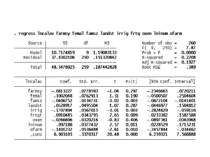
 analysis • Consider the database food_security to")
Computer Lab 1: Multiple linear regression (MLR) analysis • Consider the database food_security to estimate a linear model of determinants of daily calorie intake (lncalav). Suppose the factors influencing daily calorie intake per capita of households are farming system (farmsy), gender (femal), family size (famsz), land allocated to staples (landst), access to irrigation (irrig), fertilizer quantity used for crop production (frtqt), oxen used for draught power (oxen), (log of) annual gross income in ETB (lninom), and access to off-farm activities (ofarm). • Based on this information workout the following problems: – Estimate the OLS model for determinants of (log) daily calorie intake per adult equivalent of farm households in the study area. – Which variables are positively/adversely and significantly affecting daily calorie intake? – How do you interpret the fitness of this OLS model to identify determinants of calorie intake?

Multiple Equation Models: Multivariate regression • Multivariate regression differs from multiple regression in that several dependent variables are jointly regressed on the same independent variables. • Multivariate regression is related to Zellner’s seemingly unrelated regression, but because the same set of independent variables is used for each dependent variable. • The individual coefficients and standard errors produced are identical to those that would be produced by multiple linear regression estimating each equation separately. • The difference is that multivariate regression, being a joint estimator, also estimates the betweenequation covariances, so we can test coefficients across equations. Hence, the multivariate egression is a special case of the SUR model in which the data matrices are group-specific data sets on the same set of variables.
 • Seemingly unrelated regression (SUR) fits seemingly unrelated regression models")
Seemingly unrelated regression (SUR) • Seemingly unrelated regression (SUR) fits seemingly unrelated regression models • Seemingly unrelated regression models are so called because they appear to be joint estimates from several regression models, each with its own error term. • The regressions are related because the (contemporaneous) errors associated with the dependent variables may be correlated. • When we fit models with the same set of right-hand-side variables, the seemingly unrelated regression results (in terms of coefficients and standard errors) are the same as fitting the models separately.

Con’d • When the models do not have the same set of explanatory variables and are not nested, sureg may lead to more efficient estimates than running the models separately as well as allowing joint tests. • The seemingly unrelated regression model of two equations, y 1 and y 2 with their own separate set of explanatory variables and parameters to be estimated, can be specified as follows: y 1 = x 1β 1 + e 1 y 2 = x 2β 2 + e 2 • The syntax sureg in Stata fits seemingly unrelated regression models. sureg uses the asymptotically efficient, feasible, generalized least-squares algorithm. • The R-squared reported is the percent of variance explained by the predictors.

Computer Lab 2: Estimation and application of multiple equation models • Consider the database adoption_commercialization to estimate the multivariate regression model of market orientation of farmers in land allocation to staples food production (moist 2) and to cash crop production (moic 2). • Suppose the common explanatory variables of the two dependent variables are farming system, sex, family size, literacy status, annual gross income, number of oxen, access to irrigation, quantity of chemical fertilizer used, access to off-farm activities, access to credit, distance to the nearest market, and distance to major town. • Based on this information answer/solve the following questions/problems: – Estimate the multivariate regression model of the two equations and identify common underlying factors determining land allocation between staples and cash crops production. – Are land allocations to production of staples and cash crops interdependent household decisions?

• Answer

Con’d • According to the multivariate regression model outputs reported below, the common underlying factors determining land allocation between stapes and cash crops are family size, number of oxen, distance to the nearest market and town. • The null that the two equations are independent is rejected. • The results suggest that market orientation of farmers in their land allocation between staples and cash crops are interdependent household decisions.

Sur model: example • Consider the database Adoption and Commercialization to estimate the linear SUR model of market orientation of farmers in land allocation between staples (moist 2) and cash crops (moic 2). • Suppose the explanatory variables influencing market orientation of farmers in their land allocation between staples and cash crops are as follows: 1. moist 2 = f(sex, family size, livestock holding, access to irrigation, quantity of chemical fertilizer used, access to off-farm activities, access to credit, and access to the nearest market). 2. moic 2 = f(sex, family size, literacy status, livestock holding, access to irrigation, quantity of chemical fertilizer used, access to credit, distance to the nearest market , and distance to major town). • Based on this information do the following activities: – Estimate the linear SUR model of market orientation of farmers in land allocation between staples (moist 2) and cash crops (moic 2) and interpret the model outputs. – Are market orientation of farmers in land allocation between staples and cash crops interdependent household decisions in the study area? – Identify the common underlying factors determining land allocation between staples and cash crops production. – Predict the two dependent variables from the SUR model.

• Answer

Con’d • The SUR model outputs suggest that about 41% and 10% of the variations in land allocation between staples and cash crops are explained by the variables. • The common underlying factors determining land allocation in the study area are sex of the head, family size, distance to the nearest market and town. • The land allocation decisions of farmers between staples and cash crops are interdependent.

Con’d • The predicted values of the two dependent variables (moist 2 and moic 2) are reported below. • The market orientation index (%) of farmers in their land allocation to stapes predicted by the variables is about 52% whereas the index for cash crops is not more than 24%.

Con’d

Con’d

violation of classical assumptions Multicollinearity Nature of Multicollinearity • When two or more independent variables in a regression model are highly correlated to each other, it is difficult to determine if each of these variables, individually, has an effect on y, and to quantify the magnitude of that effect. • Intuitively, for example, if all farms in a sample that use a lot of fertilizer also apply large amounts of pesticides (and vice versa), it would be hard to tell if the observed increase in yield is due to higher fertilizer or to higher pesticide use. • In economics, when interest and inflation rates are used as independent variables, it is often hard to quantify their individual effects on the dependent variable because they are highly correlated to each other. • Mathematically, this occurs because, everything else being constant, the standard error associated to a given OLS parameter estimate will be higher if the corresponding independent variable is more highly correlated to the other independent variables in the model. • This potential problem is known as multicollinearity.
 exists when at least some of the predictor variables")
Con’d • Multicollinearity (or intercorrelation) exists when at least some of the predictor variables are correlated among themselves. In observational studies, multicollinearity happens more often than not. So, we need to understand the effects of multicollinearity on regression analyses. • When correlation among x' s is low, OLS has lots of information to estimate the coefficients. • This gives us confidence in our estimates. When correlation among x' s is high, OLS has very little information to estimate the parameters. This makes us relatively uncertain about our estimate of these parameters. • Multicollinearity could be the reason why independent variables that are believed to be key in determining the value of a given dependent variable do not result statistically significant when conducting the basic significance test. It is not a mistake in the model specification, but due to the nature of the data at hand. It is more common in time-series data models because time often affects the values taken by many of the independent variables in these types of models causing them to be highly correlated to each other A certain degree of correlation (multicollinearity) between the independent variables is normal and expected in most cases. • Multicollinearity is considered severe and becomes a problem when this correlation is high and interferes with the estimation of the model’s parameters at the desired level of statistical certainty.

Con’d • Perfect multicollinearity occurs when there is a perfect linear correlation between two or more independent variables, i. e. when an independent variable is actually a linear function of one or more of the others. It occurs, for instance, when including total annual rainfall as well as rainfall during each of the seasons as independent variables in an (annual) time series model; and when independent variable takes a constant value in all observations. • If there is perfect multicollinearity, the OLS method cannot produce parameter estimates. • All cases of perfect multicollinearity are the result of making a mistake when specifying the model and can be easily corrected by properly specifying the models. Perfect multicollinearity violates the classical assumption which specifies that no explanatory variable is a perfect linear function of any other explanatory variables. • Imperfect multicollinearity occurs when two (or more) explanatory variables are imperfectly linearly related.

The major causes of multicollinearity are the following: 1. Sampling mechanism: Poorly constructed design and measurement scheme or limited range. Poorly constructed sampling design causes correlation among x' s 2. Poorly constructed measures over-aggregate information and make cases correlate. 3. Statistical model specification: adding polynomial terms or trend indicators. 4. Too many variables in the model: x' s measure the same conceptual variable. The model is over determined. 5. The covariates, x' s , are causally related to one another. 6. Wrong theoretical specification. Inappropriate construction of theory.

high degree of multicollinearity will have the following five major consequences 1. Variance is infinite 2. Significant (high) R 2 3. Larger variance and covariances of OLS estimators 4. Wider confidence intervals 5. Variance inflation factor (VIF) Detection of High Multicollinearity • Multicollinearity is a question of degree and not of kind. • Multicollinearity is a feature of the sample and not of the population. • Therefore, we do not “test for multicollinearity” but we measure its degree in any particular sample.

Con’d Rules of thumb • High R 2 but few significant t ratios. • High pair-wise correlations among regressors. Formal test Variance inflation factor (VIF) • It is a formal test for multicollinearity is to conduct “artificial” or auxiliary regressions between each independent variable (as the “dependent” variable) and the remaining independent variables to estimate the variance inflation factors (VIFs). • VIF is a measure of the increase in the variance of the coefficient on x j due to the correlation among the explanatory variables compared to what the variance of the coefficient on x j would be if x j were independent of the other explanatory variables.

Con’d • The VIF is calculated from two steps: 1. Run an OLS regression that has xi as a function of all the other explanatory variables in the equation, this equation would be: 2. Calculate the variance inflation factor for the

Con’d • Ideally, VIFs are 1, indicating the variable provides completely independent information or no multicollinearity. • The higher the VIF, the more severe will be the effects of multicollinearity. • VIFj = 2 , for example, means that variance is twice what it would be if x j was not affected by multicollinearity. • A VIFj > 10 is clear evidence that the estimation of b j is being affected by multicollinearity

Remedial Measures for Multicollinearity • Transformation of variables • Enlarging the sample by adding new data • factor analysis, principal component and ridge regression

Illustration of Detecting Multicollinearity • Perfectly uncorrelated data

• if we regress y on x 1, we will get the following output: • If we regress y on x 2, we will get the following output:

• If we regress y on x 1 and x 2, we will get the following output:

HETEROSCEDASTICITY • The assumption of homoscedasticity is that the error variance is constant. • Homoscedasticity implies that, conditional on the explanatory variables, the variance of the error u is constant (does not depend on x): Var(ui / xi ) = constant. • If there is non-constant variance of the error terms, the error terms are related to some variable • If the variance of u is different for different values of the x' s , then the errors are heteroscedastic:

HETEROSCEDASTICITY • Heteroscedasticity may be caused by: Ø Model misspecification - omitted variable or improper functional form; Ø Learning behaviors across time; Ø Changes in data collection or definitions: Outliers or breakdown in model: Frequently observed in cross sectional data sets where demographics are involved • The consequences of heteroscedasticity are Ø OLS estimator is not of the smallest variance Ø Least square estimators are not efficient (not BLUE) Ø Hypothesis test error Ø Confidence interval of explained variable is predicted incorrectly

Graphic Detection of Heteroscedasticity: Residual plots • Homoscedastic and heteroscedastic pattern of errors

Detection of heteroscedasticity from graphic plots

Formal Tests for Heteroscedasticity •

Con’d •

Remedial Measures for Heteroscedasticity Ø In the last two decades, econometricians have learned how to adjust standard errors, so that t, F, and LM statistics are valid in the presence of heteroskedasticity. Ø This is very convenient because it means we can report new statistics that work, regardless of the kind of heteroskedasticity present in the population.

Con’d Ø While heteroscedasticity is the property of disturbances, the above tests deal with residuals. Ø Thus, they may not report the genuine heteroskedasticity. Ø Diagnostic results against homoskedasticity could be due to misspecification of the model. Ø But, if we are sure that there is a genuine heteroskedasticity problem, we can deal with the problem using: ü Heteroskedasticity-robust statistics after estimation by OLS. ü Weighted least squares (WLS) estimation.

AUTOCORRELATION •

Causes of autocorrelation Ø Specification bias Ø Cobweb phenomenon Ø Lags Ø Data manipulation Ø Nonstationarity Consequences of autocorrelation 1. the residual variance is likely to underestimate the true variance. As a result, we are likely to overestimate R 2. Therefore, the usual t and F tests of significance are no longer valid, and if applied, are likely to give seriously misleading conclusions about the statistical significance of the estimated regression coefficients. 3. The OLS estimator is no more BLUE

Detection of Autocorrelation •

Causes of autocorrelation • Specification bias • Cobweb phenomenon • Lags • Data manipulation • Nonstationarity Consequences of autocorrelation • the usual t and F tests of significance are no longer valid, • The OLS estimator is no more BLUE • confidence intervals are likely to be wider

Detection of Autocorrelation • Graphical method
 test")
Durbin-Watson (DW) test

Con’d • the Durbin Watson test relies on the following assumptions: – The regression model includes the intercept term. – The explanatory variables are non-stochastic, or fixed in repeated sampling. – The disturbances are generated by the first order autoregressive scheme. – The error term is assumed to be normally distributed. – The regression model does not include the lagged values of the dependent and explanatory variables. – There are no missing values in the data.

Con’d
 test • There are various higher")
Higher order tests: The Breusch – Godfrey (BG) test • There are various higher order tests including the Ljung-Box Q (P 2 statistic), Portmanteau test, and Breusch-Godfrey (BG) test. • The BG test, also known as the LM test, is a general test for autocorrelation in the sense that it allows for: a. nonstochastic regressors such as the lagged values of the regressand; b. higher-order autoregressive schemes such as AR(1), AR (2)etc. ; and c. simple or higher-order moving averages of white noise error terms.
 • Consider the database food_security to estimate a")
Computer Lab: Postestimation tests (after MLR) • Consider the database food_security to estimate a linear model of determinants of daily calorie intake (lncalav). Suppose the factors influencing daily calorie intake per capita of households are farming system (farmsy), gender (femal), family size (famsz), land allocated to staples (landst), access to irrigation (irrig), fertilizer quantity used for crop production (frtqt), oxen used for draught power (oxen), (log of) annual gross income in ETB (lninom), and access to off-farm activities (ofarm). workout the following problems: a. Estimate the OLS model for determinants of (log) daily calorie intake per adult equivalent of farm households in the study area. b. Are the residuals from the model estimation homoscedastic (of the same variance)? c. Is there specification error or omitted variable bias in the model? d. Are the explanatory variables seriously correlated among each other? e. Predict the daily calorie intake of all sample households and of those households with and without access to irrigation. Which predicted value is greater? Interpret the results.

The following post-estimation commands are of special interest after regress:

Tests for heteroscedasticity • The test for heteroscedasticity after OLS suggests that the errors are of the same variance. The null that the errors have constant variance is accepted. Testes for omitted variables • The null that there is not omitted variable in the model is accepted suggesting that the model has no problem of omitted variable bias.

• Tests for multicollinearity • The test for multicollinearity reported below suggests that there is no serious problem of multicollinearity among explanatory variables because the mean VIF is about 1. 6.

Predicted value • The predicted value of the dependent variable is about 7. 54. The antilog of this predicted value is 1878. 7 kcal, suggesting that households obtain this quantity of daily calorie intake as predicted by all the variables.
- Slides: 118