Econometrics Econ 504 Chapter 8 DUMMY VARIABLE D

Econometrics Econ. 504 Chapter 8: DUMMY VARIABLE (D. V. ) REGRESSION MODELS

I. The Natural of Dummy Variables § In regression analysis the dependent variable is frequently influenced by variables that are essentially qualitative, in nature, such as sex, race, color, religion, nationality, geographical region, etc. § One way we could “quantify” such attributes is by constructing artificial variables such that: Ø 1 indicating the presence of that attribute. Ø 0 indicating the absence of that attribute.

§ Variables that assume such 0 and 1 values are called dummy variables. § Example: (A) “ 1” may indicate that a person is a female and 0 may designate a male; (B) “ 1” may indicate that a person is a college graduate, and 0 that the person is not, and so on.

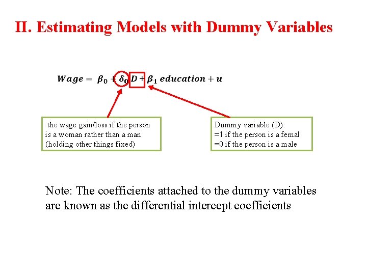
II. Estimating Models with Dummy Variables the wage gain/loss if the person is a woman rather than a man (holding other things fixed) Dummy variable (D): =1 if the person is a femal =0 if the person is a male Note: The coefficients attached to the dummy variables are known as the differential intercept coefficients

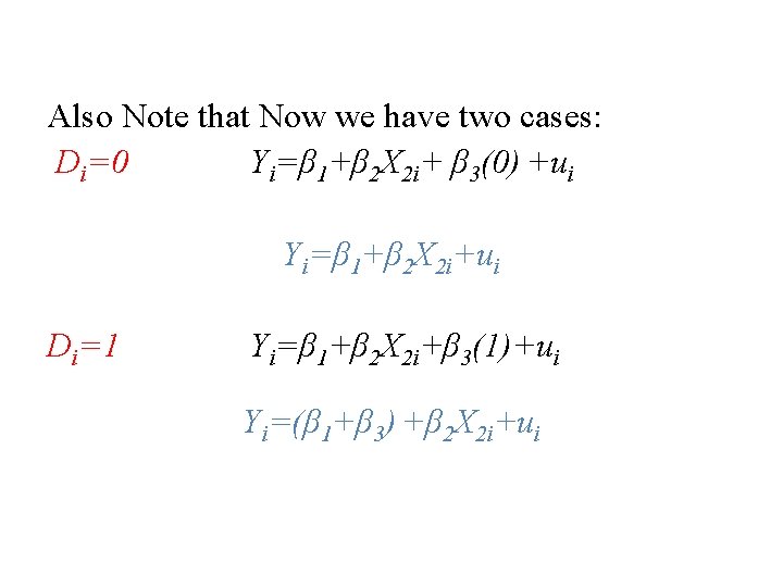
Also Note that Now we have two cases: Di=0 Yi=β 1+β 2 X 2 i+ β 3(0) +ui Yi=β 1+β 2 X 2 i+ui Di=1 Yi=β 1+β 2 X 2 i+β 3(1)+ui Yi=(β 1+β 3) +β 2 X 2 i+ui

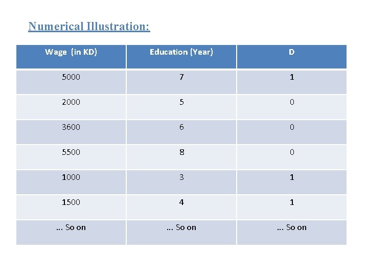
Numerical Illustration: Wage (in KD) Education (Year) D 5000 7 1 2000 5 0 3600 6 0 5500 8 0 1000 3 1 1500 4 1 . . . So on

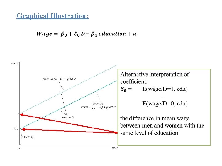
Graphical Illustration:

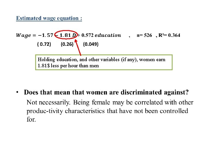
• Holding education, and other variables (if any), women earn 1. 81$ less per hour than men

II. Caution in the Use of Dummy Variables § When dealing with dummy variables in the regression function, you should be aware to some important aspects. § Therefore, there are three forms of model that are used to explain the multiple regression analysis with qualitative information.

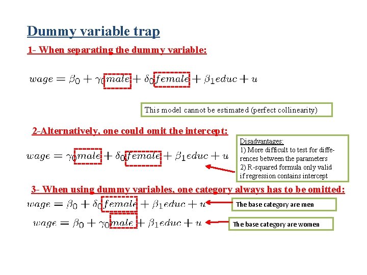
Dummy variable trap 1 - When separating the dummy variable: This model cannot be estimated (perfect collinearity) 2 -Alternatively, one could omit the intercept: Disadvantages: 1) More difficult to test for differences between the parameters 2) R-squared formula only valid if regression contains intercept 3 - When using dummy variables, one category always has to be omitted: The base category are men The base category are women

III. Interaction Variables § We can use dummy variables as standalone independent variables, but also we can interact (multiply) them with quantitative variables. § Interacting dummy variables with quantitative variables provides flexibility to detect differences between groups overall and differences that may vary depending on the value of quantitative variables.

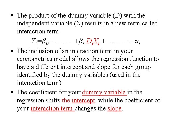
§ The product of the dummy variable (D) with the independent variable (X) results in a new term called interaction term: Yi=β 0+………+βi Di. Xi + ………+ ui § The inclusion of an interaction term in your econometrics model allows the regression function to have a different intercept and slope for each group identified by the dummy variables (used in the interaction term). § The coefficient for your dummy variable in the regression shifts the intercept, while the coefficient of your interaction term changes the slope.

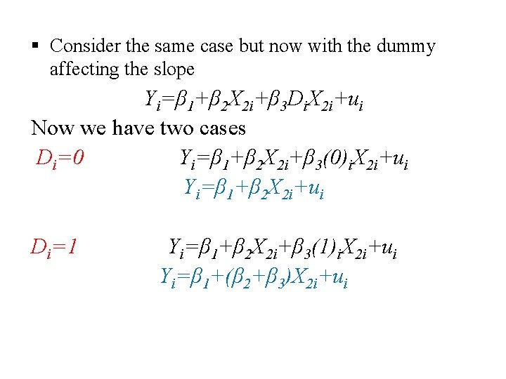
§ Consider the same case but now with the dummy affecting the slope Yi=β 1+β 2 X 2 i+β 3 Di. X 2 i+ui Now we have two cases Di=0 Yi=β 1+β 2 X 2 i+β 3(0)i. X 2 i+ui Yi=β 1+β 2 X 2 i+ui Di=1 Yi=β 1+β 2 X 2 i+β 3(1)i. X 2 i+ui Yi=β 1+(β 2+β 3)X 2 i+ui

IV. Testing of Significance § When using dummy variables in the regression, you have to take into account the collective significance of those variables. § Their effect can be collectively significant even if they are individually insignificant.

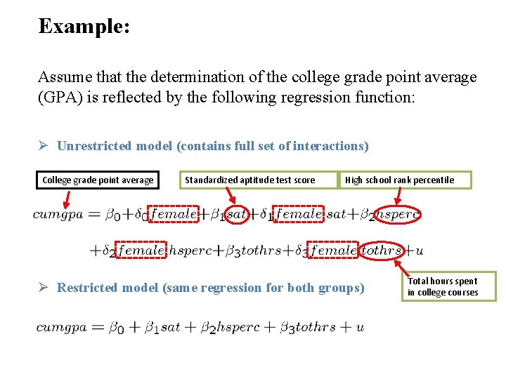
Example: Assume that the determination of the college grade point average (GPA) is reflected by the following regression function: Ø Unrestricted model (contains full set of interactions) College grade point average Standardized aptitude test score High school rank percentile Ø Restricted model (same regression for both groups) Total hours spent in college courses

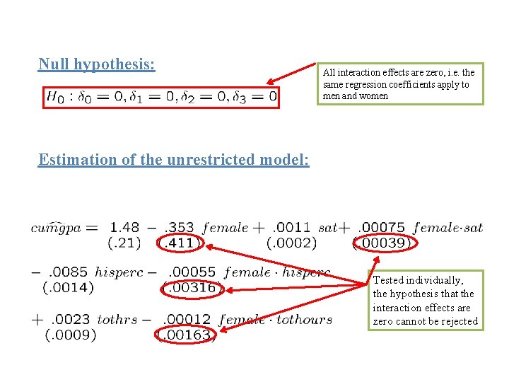
Null hypothesis: All interaction effects are zero, i. e. the same regression coefficients apply to men and women Estimation of the unrestricted model: Tested individually, the hypothesis that the interaction effects are zero cannot be rejected

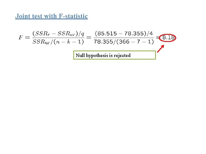
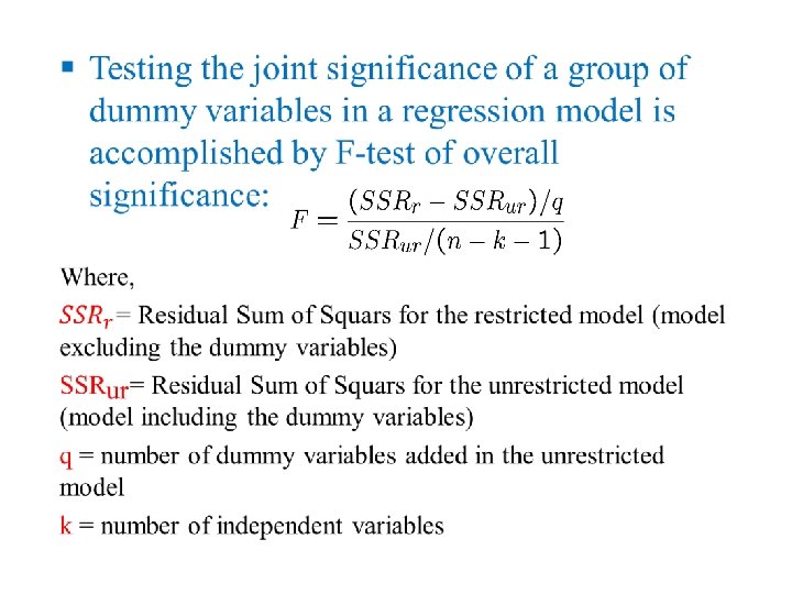
Joint test with F-statistic Null hypothesis is rejected

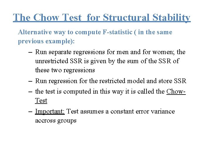
The Chow Test for Structural Stability Alternative way to compute F-statistic ( in the same previous example): – Run separate regressions for men and for women; the unrestricted SSR is given by the sum of the SSR of these two regressions – Run regression for the restricted model and store SSR – the test is computed in this way it is called the Chow. Test – Important: Test assumes a constant error variance accross groups

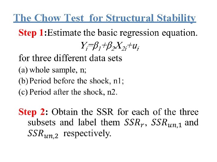
The Chow Test for Structural Stability •

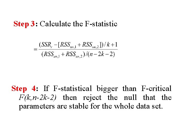
Step 3: Calculate the F-statistic Step 4: If F-statistical bigger than F-critical F(k, n-2 k-2) then reject the null that the parameters are stable for the whole data set.