Econometrics 2 Lecture 6 Models Based on Panel

Econometrics 2 - Lecture 6 Models Based on Panel Data

Contents n n n n Panel Data Pooling Independent Cross-sectional Data Panel Data: Pooled OLS Estimation Panel Data Models Fixed Effects Model Random Effects Model Analysis of Panel Data Models Panel Data in GRETL April 19, 2013 Hackl, Econometrics 2, Lecture 6 2

Types of Data Population of interest: individuals, households, companies, countries Types of observations n Cross-sectional data: observations of all units of a population, or of a representative subset, at one specific point in time n Time series data: series of observations on units of the population over a period of time n Panel data (longitudinal data): repeated observations of (the same) population units collected over a number of periods; data set with both a cross-sectional and a time series aspect; multi-dimensional data Cross-sectional and time series data are one-dimensional, special cases of panel data Pooling independent cross-sections: (only) similar to panel data April 19, 2013 Hackl, Econometrics 2, Lecture 6 3

Example: Individual Wages Verbeek’s data set “males” n Sample of n 545 full-time working males each person observed yearly after completion of school in 1980 till 1987 Variables wage: log of hourly wage (in USD) school: years of schooling exper: age – 6 – school dummies for union membership, married, black, Hispanic, public sector others April 19, 2013 Hackl, Econometrics 2, Lecture 6 4

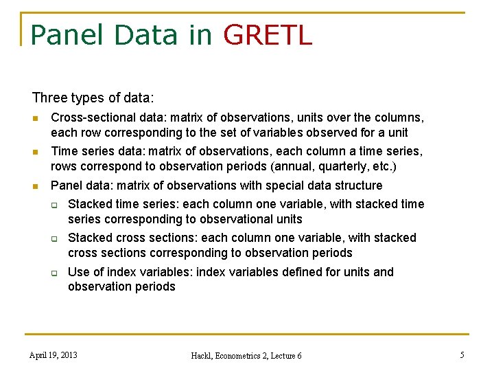
Panel Data in GRETL Three types of data: n Cross-sectional data: matrix of observations, units over the columns, each row corresponding to the set of variables observed for a unit n Time series data: matrix of observations, each column a time series, rows correspond to observation periods (annual, quarterly, etc. ) n Panel data: matrix of observations with special data structure Stacked time series: each column one variable, with stacked time series corresponding to observational units Stacked cross sections: each column one variable, with stacked cross sections corresponding to observation periods Use of index variables: index variables defined for units and observation periods April 19, 2013 Hackl, Econometrics 2, Lecture 6 5

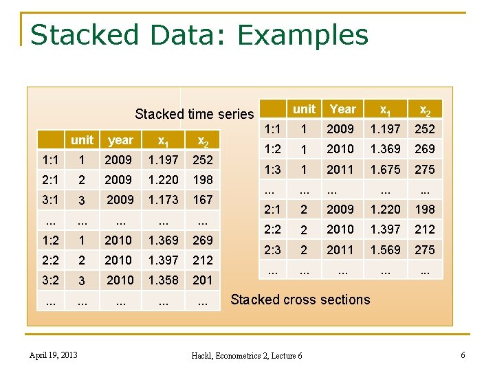
Stacked Data: Examples Stacked time series unit year x 1 x 2 1: 1 1 2009 1. 197 252 2: 1 2 2009 1. 220 198 3: 1 3 2009 1. 173 167 . . . . 1 2010 1. 369 269 1: 2 2 2010 1. 397 212 3: 2 3 2010 1. 358 201 . . . . April 19, 2013 unit Year x 1 x 2 1: 1 1 2009 1. 197 252 1: 2 1 2010 1. 369 269 1: 3 1 2011 1. 675 275 . . . . 2: 1 2 2009 1. 220 198 2: 2 2 2010 1. 397 212 2: 3 2 2011 1. 569 275 . . . . Stacked cross sections Hackl, Econometrics 2, Lecture 6 6

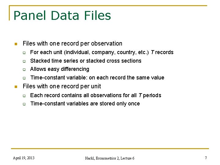
Panel Data Files n n Files with one record per observation For each unit (individual, company, country, etc. ) T records Stacked time series or stacked cross sections Allows easy differencing Time-constant variable: on each record the same value Files with one record per unit Each record contains all observations for all T periods Time-constant variables are stored only once April 19, 2013 Hackl, Econometrics 2, Lecture 6 7

Panel Data Typically data at micro-economic level (individuals, households, firms), but also at macro-economic level (e. g. , countries) Notation: n N: Number of cross-sectional units n T: Number of time periods Types of panel data: n Large T, small N: “long and narrow” n Small T, large N: “short and wide” n Large T, large N: “long and wide” Example: Data set “males”: short (T = 8) and wide (N = 545) panel (N » T) April 19, 2013 Hackl, Econometrics 2, Lecture 6 8

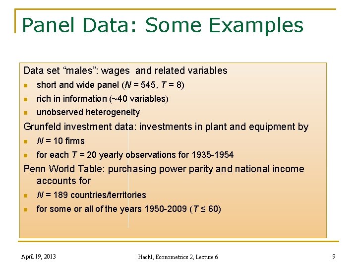
Panel Data: Some Examples Data set “males”: wages and related variables n short and wide panel (N = 545, T = 8) n rich in information (~40 variables) n unobserved heterogeneity Grunfeld investment data: investments in plant and equipment by n N = 10 firms n for each T = 20 yearly observations for 1935 -1954 Penn World Table: purchasing power parity and national income accounts for n N = 189 countries/territories n for some or all of the years 1950 -2009 (T ≤ 60) April 19, 2013 Hackl, Econometrics 2, Lecture 6 9

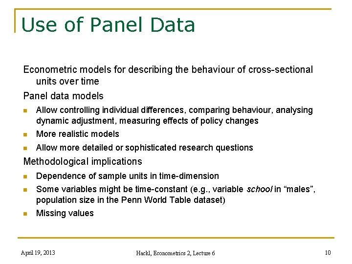
Use of Panel Data Econometric models for describing the behaviour of cross-sectional units over time Panel data models n Allow controlling individual differences, comparing behaviour, analysing dynamic adjustment, measuring effects of policy changes n More realistic models n Allow more detailed or sophisticated research questions Methodological implications n Dependence of sample units in time-dimension n Some variables might be time-constant (e. g. , variable school in “males”, population size in the Penn World Table dataset) n Missing values April 19, 2013 Hackl, Econometrics 2, Lecture 6 10

Contents n n n n Panel Data Pooling Independent Cross-sectional Data Panel Data: Pooled OLS Estimation Panel Data Models Fixed Effects Model Random Effects Model Analysis of Panel Data Models Panel Data in GRETL April 19, 2013 Hackl, Econometrics 2, Lecture 6 11

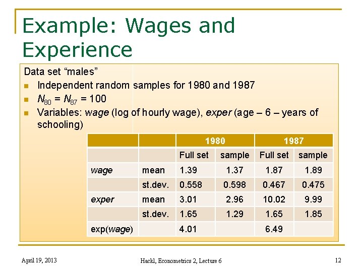
Example: Wages and Experience Data set “males” n Independent random samples for 1980 and 1987 n N 80 = N 87 = 100 n Variables: wage (log of hourly wage), exper (age – 6 – years of schooling) 1980 Full set wage exper exp(wage) April 19, 2013 1987 sample Full set sample mean 1. 39 1. 37 1. 89 st. dev. 0. 558 0. 598 0. 467 0. 475 mean 3. 01 2. 96 10. 02 9. 99 st. dev. 1. 65 1. 29 1. 65 1. 85 4. 01 Hackl, Econometrics 2, Lecture 6 6. 49 12

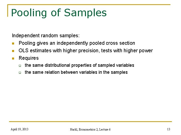
Pooling of Samples Independent random samples: n Pooling gives an independently pooled cross section n n OLS estimates with higher precision, tests with higher power Requires the same distributional properties of sampled variables the same relation between variables in the samples April 19, 2013 Hackl, Econometrics 2, Lecture 6 13

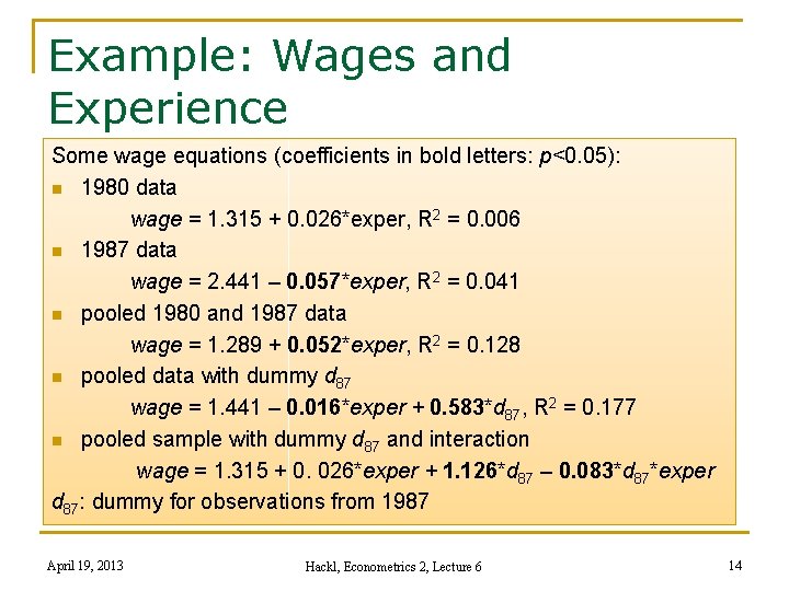
Example: Wages and Experience Some wage equations (coefficients in bold letters: p<0. 05): n 1980 data wage = 1. 315 + 0. 026*exper, R 2 = 0. 006 n 1987 data wage = 2. 441 – 0. 057*exper, R 2 = 0. 041 n pooled 1980 and 1987 data wage = 1. 289 + 0. 052*exper, R 2 = 0. 128 n pooled data with dummy d 87 wage = 1. 441 – 0. 016*exper + 0. 583*d 87, R 2 = 0. 177 n pooled sample with dummy d 87 and interaction wage = 1. 315 + 0. 026*exper + 1. 126*d 87 – 0. 083*d 87*exper d 87: dummy for observations from 1987 April 19, 2013 Hackl, Econometrics 2, Lecture 6 14

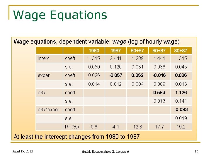
Wage Equations Wage equations, dependent variable: wage (log of hourly wage) Interc. exper d 87*exper 1980 1987 80+87 coeff 1. 315 2. 441 1. 289 1. 441 1. 315 s. e. 0. 050 0. 120 0. 031 0. 036 0. 045 coeff 0. 026 -0. 057 0. 052 -0. 016 0. 026 s. e. 0. 014 0. 012 0. 004 0. 009 0. 013 coeff 0. 583 1. 126 s. e. 0. 073 0. 141 coeff -0. 083 s. e. 0. 019 R 2 (%) 0. 6 4. 1 12. 8 17. 7 19. 2 At least the intercept changes from 1980 to 1987 April 19, 2013 Hackl, Econometrics 2, Lecture 6 15

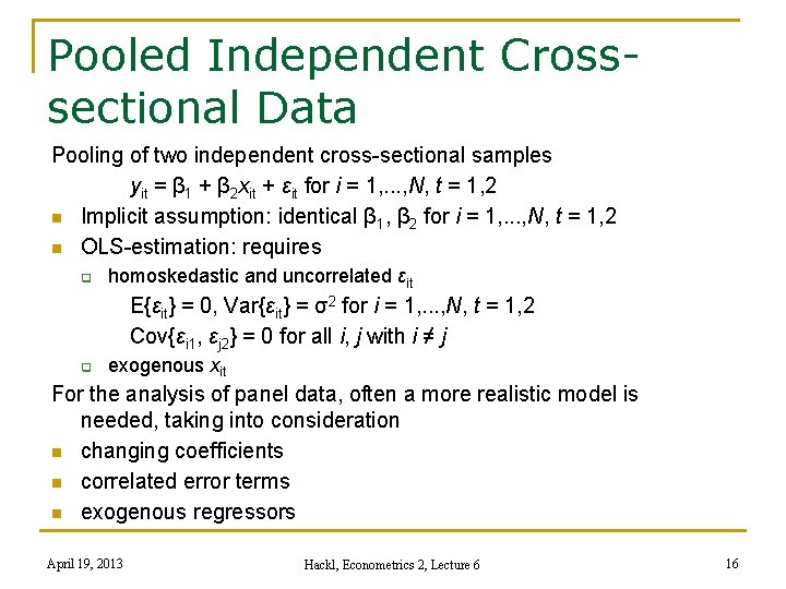
Pooled Independent Crosssectional Data Pooling of two independent cross-sectional samples yit = β 1 + β 2 xit + εit for i = 1, . . . , N, t = 1, 2 n Implicit assumption: identical β 1, β 2 for i = 1, . . . , N, t = 1, 2 n OLS-estimation: requires homoskedastic and uncorrelated εit E{εit} = 0, Var{εit} = σ2 for i = 1, . . . , N, t = 1, 2 Cov{εi 1, εj 2} = 0 for all i, j with i ≠ j exogenous xit For the analysis of panel data, often a more realistic model is needed, taking into consideration n changing coefficients n correlated error terms n exogenous regressors April 19, 2013 Hackl, Econometrics 2, Lecture 6 16

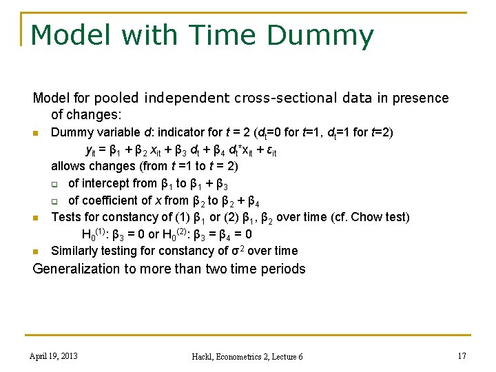
Model with Time Dummy Model for pooled independent cross-sectional data in presence of changes: n n n Dummy variable d: indicator for t = 2 (dt=0 for t=1, dt=1 for t=2) yit = β 1 + β 2 xit + β 3 dt + β 4 dt*xit + εit allows changes (from t =1 to t = 2) of intercept from β 1 to β 1 + β 3 of coefficient of x from β 2 to β 2 + β 4 Tests for constancy of (1) β 1 or (2) β 1, β 2 over time (cf. Chow test) H 0(1): β 3 = 0 or H 0(2): β 3 = β 4 = 0 Similarly testing for constancy of σ2 over time Generalization to more than two time periods April 19, 2013 Hackl, Econometrics 2, Lecture 6 17

Example: Wages and Experience Wage equation wageit = β 1 + β 2 experit + β 3 dt + εit Wages might depend also on other variables; omitted variables are covered by the error terms n black: time-constant variable, omission may cause autocorrelation of error terms; similar other time-constant factors like hisp n mar (married): variable which is for many (not all) units timeconstant, similar rural, union, ne (living in north east), etc. ; omission may cause autocorrelation n school: omission may cause endogeneity of exper n Unobserved and unobservable variables can have similar effects, e. g. , parental background, attitudes, etc. April 19, 2013 Hackl, Econometrics 2, Lecture 6 18

Problems with Sample Pooling The analysis of the data (yit, xit), i = 1, . . . , N, t = 1, 2, by OLS estimation of the parameters of model yit = β 1 + β 2 xit + εit (or extensions based on a year dummy for t=2) may not fulfil usual requirements n The independence assumption across time may be unrealistic n Main reason is that effects of non-measured and non-measurable variables are only covered by the error terms n Also exogeneity of regressors may be unrealistic Consequences: OLS-estimates n biased and inconsistent n not efficient Panel data models allow more adequate analyses April 19, 2013 Hackl, Econometrics 2, Lecture 6 19

Contents n n n n Panel Data Pooling Independent Cross-sectional Data Panel Data: Pooled OLS Estimation Panel Data Models Fixed Effects Model Random Effects Model Analysis of Panel Data Models Panel Data in GRETL April 19, 2013 Hackl, Econometrics 2, Lecture 6 20

Models for Panel Data Model for y, based on panel data from N cross-sectional units and T periods yit = β 0 + xit’β 1 + εit i = 1, . . . , N: sample unit t = 1, . . . , T: time period of sample xit and β 1: K-vectors n β 0 and β 1: represent intercept and K regression coefficients; are assumed to be identical for all units and all time periods n εit: represents unobserved factors that may affect yit Assumption that εit are uncorrelated over time not realistic Standard errors of OLS estimates misleading, OLS estimation not efficient April 19, 2013 Hackl, Econometrics 2, Lecture 6 21

Fixed Effects Model The general model yit = β 0 + xit’β 1 + εit n Specification for the error terms: two components εit = αi + uit n n αi unit-specific, time-constant factors, also called unobserved (individual) heterogeneity; may be correlated with xit uit ~ IID(0, σu 2); uncorrelated over time; represents unobserved factors that change over time, also called idiosyncratic or timevarying error εit : also called composite error Fixed effects (FE) model yit = Σj αi dij + xit’β 1 + uit dij: dummy variable for unit i: dij = 1 if i = j, otherwise dij = 0 Overall intercept omitted; unit-specific intercepts αi April 19, 2013 Hackl, Econometrics 2, Lecture 6 22

Random Effects Model Starting point is again the model yit = β 0 + xit’β 1 + εit with composite error εit = αi + uit n Specification for the error terms: n n n uit ~ IID(0, σu 2); uncorrelated over time αi ~ IID(0, σa 2); represents all unit-specific, time-constant factors; correlation of error terms over time only via the αi αi and uit are assumed to be mutually independent and independent of xjs for all j and s Random effects (RE) model yit = β 0 + xit’β 1 + αi + uit Unbiased and consistent (N → ∞) estimation of β 0 and β 1 Efficient estimation of β 0 and β 1: takes error covariance structure into account; GLS estimation April 19, 2013 Hackl, Econometrics 2, Lecture 6 23

Contents n n n n Panel Data Pooling Independent Cross-sectional Data Panel Data: Pooled OLS Estimation Panel Data Models Fixed Effects Model Random Effects Model Analysis of Panel Data Models Panel Data in GRETL April 19, 2013 Hackl, Econometrics 2, Lecture 6 24

Fixed Effects (FE) Model for y, based on panel data for T periods yit = αi + xit’β + uit , uit ~ IID(0, σu 2) i = 1, . . . , N: sample unit t = 1, . . . , T: time period of sample n αi: fixed parameter, represents all unit-specific, time-constant factors, unobserved (individual) heterogeneity n xit: all K components are assumed to be independent of all uit; may be correlated with αi Model with dummies dij = 1 for i = j and 0 otherwise: yit = Σj αi dij + xit’β + uit n Number of coefficients: N + K n Main interest: estimators for β April 19, 2013 Hackl, Econometrics 2, Lecture 6 25

FE Model Parameters: Estimation FE model with dummies dij = 1 for i = j and 0 otherwise: yit = Σj αi dij + xit’β + uit Number of coefficients: N + K Various estimation procedures are available n Least squares dummy variable (LSDV) estimator n Within or fixed effects estimator n First-difference estimator A special case n Differences-in-differences (DD or DID or D-in-D) estimator April 19, 2013 Hackl, Econometrics 2, Lecture 6 26

Least Squares Dummy Variable (LSDV) Estimator Estimation procedure for N + K parameters β and αi of the FE model yit = Σj αi dij + xit’β + uit OLS estimation n NT observations for estimating N + K coefficients n Numerically costly, not attractive n Estimates for αi usually not of interest Fixed effects and first-difference estimators are more attractive April 19, 2013 Hackl, Econometrics 2, Lecture 6 27

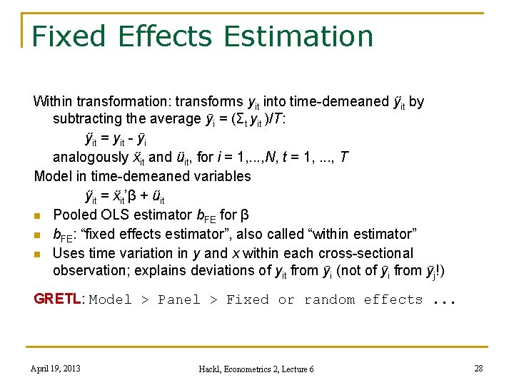
Fixed Effects Estimation Within transformation: transforms yit into time-demeaned ÿit by subtracting the average ӯi = (Σt yit )/T: ÿit = yit - ӯi analogously ẍit and üit, for i = 1, . . . , N, t = 1, . . . , T Model in time-demeaned variables ÿit = ẍit’β + üit n Pooled OLS estimator b. FE for β n b. FE: “fixed effects estimator”, also called “within estimator” n Uses time variation in y and x within each cross-sectional observation; explains deviations of yit from ӯi (not of ӯi from ӯj!) GRETL: Model > Panel > Fixed or random effects. . . April 19, 2013 Hackl, Econometrics 2, Lecture 6 28

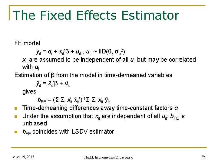
The Fixed Effects Estimator FE model yit = αi + xit’β + uit , uit ~ IID(0, σu 2) xit are assumed to be independent of all uit but may be correlated with αi Estimation of β from the model in time-demeaned variables ÿit = ẍit’β + üit gives b. FE = (Σj Σt ẍit’)-1Σj Σt ẍit ÿit n Time-demeaning differences away time-constant factors αi n Under the assumption that xit are independent of all uit: b. FE is unbiased n b. FE coincides with LSDV estimator April 19, 2013 Hackl, Econometrics 2, Lecture 6 29

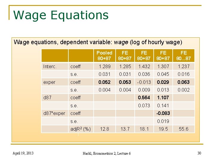
Wage Equations Wage equations, dependent variable: wage (log of hourly wage) Interc. exper d 87*exper Pooled 80+87 FE 80. . . 87 coeff 1. 289 1. 285 1. 432 1. 307 1. 237 s. e. 0. 031 0. 036 0. 045 0. 016 coeff 0. 052 0. 053 -0. 013 0. 029 0. 063 s. e. 0. 004 0. 009 0. 013 0. 002 coeff 0. 564 1. 107 s. e. 0. 073 0. 141 coeff -0. 083 s. e. 0. 019 adj. R 2 (%) April 19, 2013 12. 8 13. 7 Hackl, Econometrics 2, Lecture 6 18. 1 19. 5 55. 6 30

Properties of Fixed Effects Estimator n n n n b. FE = (ΣiΣt ẍit’)-1 ΣiΣt ẍit ÿit Unbiased if all xit are independent of all uit Normally distributed if normality of uit is assumed Consistent (for N → ∞) if xit are strictly exogenous, i. e. , E{xit uis} = 0 for all s, t Asymptotically normally distributed Covariance matrix V{b. FE} = σu 2(ΣiΣt ẍit’)-1 Estimated covariance matrix: substitution of σu 2 by su 2 = (ΣiΣt ῦitῦit)/[N(T-1)] with the residuals ῦit = ÿit - ẍit’b. FE Attention! The standard OLS estimate of the covariance matrix underestimates the true values April 19, 2013 Hackl, Econometrics 2, Lecture 6 31

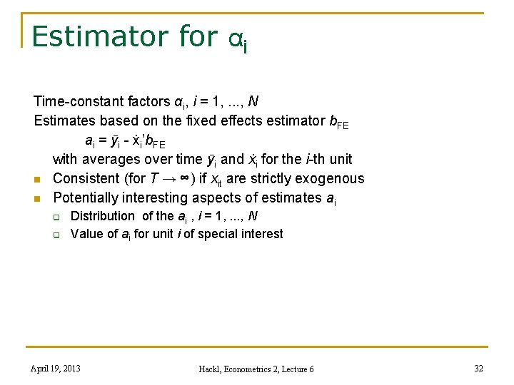
Estimator for αi Time-constant factors αi, i = 1, . . . , N Estimates based on the fixed effects estimator b. FE ai = ӯi - ẋi’b. FE with averages over time ӯi and ẋi for the i-th unit n Consistent (for T → ∞) if xit are strictly exogenous n Potentially interesting aspects of estimates ai Distribution of the ai , i = 1, . . . , N Value of ai for unit i of special interest April 19, 2013 Hackl, Econometrics 2, Lecture 6 32

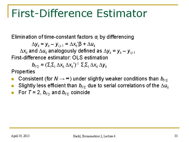
First-Difference Estimator Elimination of time-constant factors αi by differencing ∆yit = yit – yi, t-1 = ∆xit’β + ∆uit ∆xit and ∆uit analogously defined as ∆yit = yit – yi, t-1 First-difference estimator: OLS estimation b. FD = (ΣiΣt ∆xit’)-1 ΣiΣt ∆xit ∆yit Properties n Consistent (for N → ∞) under slightly weaker conditions than b. FE n Slightly less efficient than b. FE due to serial correlations of the ∆uit n For T = 2, b. FD and b. FE coincide April 19, 2013 Hackl, Econometrics 2, Lecture 6 33

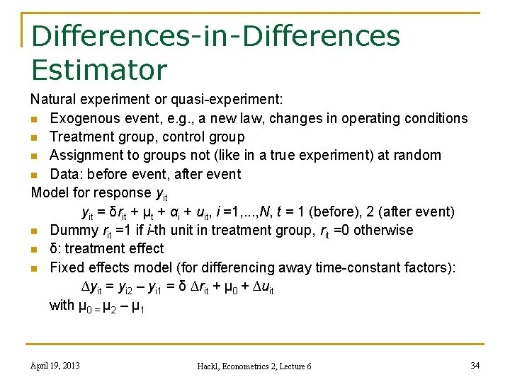
Differences-in-Differences Estimator Natural experiment or quasi-experiment: n Exogenous event, e. g. , a new law, changes in operating conditions n Treatment group, control group n Assignment to groups not (like in a true experiment) at random n Data: before event, after event Model for response yit = δrit + μt + αi + uit, i =1, . . . , N, t = 1 (before), 2 (after event) n Dummy rit =1 if i-th unit in treatment group, rit =0 otherwise n δ: treatment effect n Fixed effects model (for differencing away time-constant factors): ∆yit = yi 2 – yi 1 = δ ∆rit + μ 0 + ∆uit with μ 0 = μ 2 – μ 1 April 19, 2013 Hackl, Econometrics 2, Lecture 6 34

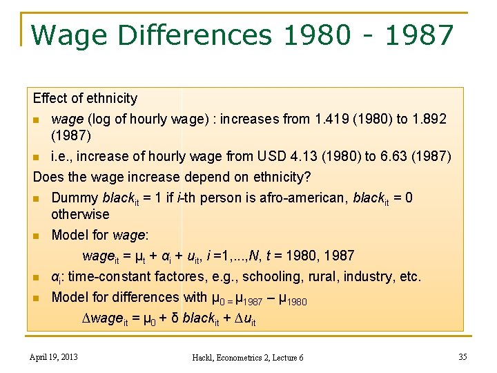
Wage Differences 1980 - 1987 Effect of ethnicity n wage (log of hourly wage) : increases from 1. 419 (1980) to 1. 892 (1987) n i. e. , increase of hourly wage from USD 4. 13 (1980) to 6. 63 (1987) Does the wage increase depend on ethnicity? n Dummy blackit = 1 if i-th person is afro-american, blackit = 0 otherwise n Model for wage: wageit = μt + αi + uit, i =1, . . . , N, t = 1980, 1987 n αi: time-constant factores, e. g. , schooling, rural, industry, etc. n Model for differences with μ 0 = μ 1987 – μ 1980 ∆wageit = μ 0 + δ blackit + ∆uit April 19, 2013 Hackl, Econometrics 2, Lecture 6 35

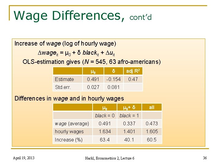
Wage Differences, cont’d Increase of wage (log of hourly wage) ∆wageit = μ 0 + δ blackit + ∆uit OLS-estimation gives (N = 545, 63 afro-americans) μ 0 δ adj R 2 Estimate 0. 491 -0. 154 0. 47 Std. err. 0. 027 0. 081 Differences in wage and in hourly wages μ 0+ δ all black = 0 black = 1 April 19, 2013 wage (average) 0. 491 0. 337 0. 473 hourly wages 1. 634 1. 401 1. 605 Increase (%) 63. 4 40. 1 60. 5 Hackl, Econometrics 2, Lecture 6 36

Estimator of Treatment Effect of treatment (event) by comparing units with and without treatment before and after treatment Model for panel data yit = δrit + μt + αi + uit, i =1, . . . , N, t = 1 (before), 2 (after event) Differences-in-differences (DD or DID or D-in-D) estimator of treatment effect δ d. DD = ∆ӯtreated - ∆ӯuntreated ∆ӯtreated: average difference yi 2 – yi 1 of treatment group units ∆ӯuntreated: average difference yi 2 – yi 1 of control group units n Treatment effect δ measured as difference between changes of y with and without treatment n d. DD consistent if E{∆rit ∆uit} = 0 n Allows correlation between time-constant factors αi and rit April 19, 2013 Hackl, Econometrics 2, Lecture 6 37

Contents n n n n Panel Data Pooling Independent Cross-sectional Data Panel Data: Pooled OLS Estimation Panel Data Models Fixed Effects Model Random Effects Model Analysis of Panel Data Models Panel Data in GRETL April 19, 2013 Hackl, Econometrics 2, Lecture 6 38

Random Effects Model: n n n yit = β 0 + xit’β + αi + uit , uit ~ IID(0, σu 2) Time-constant factors αi: stochastic variables with identical distribution for all units αi ~ IID(0, σa 2) Attention! More information about αi than in the fixed effects model αi + uit: error term with two components n n Unit-specific component αi, time-constant Remainder uit, assumed to be uncorrelated over time αi, uit: mutually independent, independent of xjs for all j and s OLS estimators for β 0 and β are unbiased, consistent, not efficient (see next slide) April 19, 2013 Hackl, Econometrics 2, Lecture 6 39

GLS Estimator αi i. T + ui: T-vector of error terms for i-th unit, T-vector i. T = (1, . . . , 1)’ Ω = Var{αii. T + ui}: Covariance matrix of αii. T + ui Ω = σa 2 i. T’ + σu 2 IT Inverted covariance matrix Ω-1 = σu-2{[IT – (i. T’)/T] + ψ (i. T’)/T} with ψ = σu 2/(σu 2 + Tσa 2) (i. T’)/T: transforms into averages IT – (i. T’)/T: transforms into deviations from average GLS estimator b. GLS = [ΣiΣtẍitẍit’+ψTΣi(ẋi –ẋ)’]-1[ΣiΣtẍitÿit+ψTΣi(ẋi –ẋ)(ӯi –ӯ)] with the average ӯ over all i and t, analogous ẋ n ψ = 0: b. GLS coincides with b. FE; b. GLS and b. FE equivalent for large T n ψ = 1: b. GLS coincides with the OLS estimators for β 0 and β April 19, 2013 Hackl, Econometrics 2, Lecture 6 40

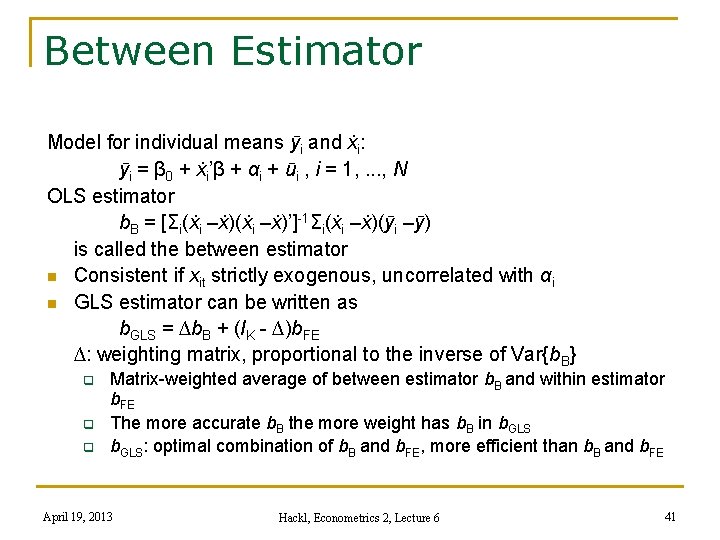
Between Estimator Model for individual means ӯi and ẋi: ӯi = β 0 + ẋi’β + αi + ūi , i = 1, . . . , N OLS estimator b. B = [Σi(ẋi –ẋ)’]-1Σi(ẋi –ẋ)(ӯi –ӯ) is called the between estimator n Consistent if xit strictly exogenous, uncorrelated with αi n GLS estimator can be written as b. GLS = ∆b. B + (IK - ∆)b. FE ∆: weighting matrix, proportional to the inverse of Var{b. B} Matrix-weighted average of between estimator b. B and within estimator b. FE The more accurate b. B the more weight has b. B in b. GLS: optimal combination of b. B and b. FE, more efficient than b. B and b. FE April 19, 2013 Hackl, Econometrics 2, Lecture 6 41

GLS Estimator: Properties n n b. GLS = [ΣiΣtẍitẍit’+ψTΣi(ẋi –ẋ)’]-1[ΣiΣtẍitÿit+ψTΣi(ẋi –ẋ)(ӯi –ӯ)] Unbiased, if xit are independent of all αi and uit Consistent for N or T or both tending to infinity if n E{ẍit uit} = 0 E{ẋi uit} = 0, E{ẍit αi} = 0 These conditions are required also for consistency of b. B More efficient than the between estimator b. B and the within estimator b. FE; also more efficient than the OLS estimator April 19, 2013 Hackl, Econometrics 2, Lecture 6 42

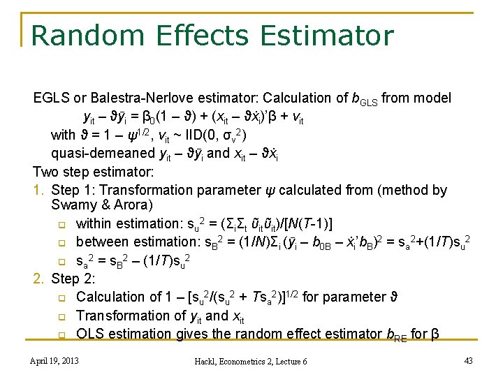
Random Effects Estimator EGLS or Balestra-Nerlove estimator: Calculation of b. GLS from model yit – ϑӯi = β 0(1 – ϑ) + (xit – ϑẋi)’β + vit with ϑ = 1 – ψ1/2, vit ~ IID(0, σv 2) quasi-demeaned yit – ϑӯi and xit – ϑẋi Two step estimator: 1. Step 1: Transformation parameter ψ calculated from (method by Swamy & Arora) within estimation: su 2 = (ΣiΣt ῦitῦit)/[N(T-1)] between estimation: s. B 2 = (1/N)Σi (ӯi – b 0 B – ẋi’b. B)2 = sa 2+(1/T)su 2 sa 2 = s. B 2 – (1/T)su 2 2. Step 2: Calculation of 1 – [su 2/(su 2 + Tsa 2)]1/2 for parameter ϑ Transformation of yit and xit OLS estimation gives the random effect estimator b. RE for β April 19, 2013 Hackl, Econometrics 2, Lecture 6 43

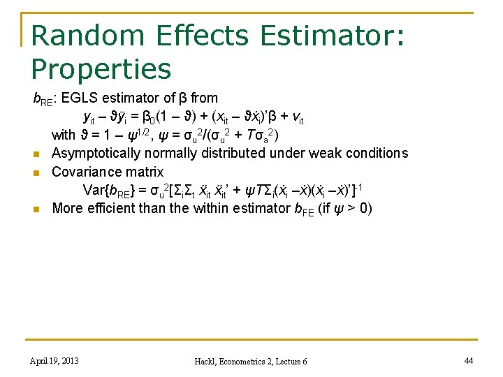
Random Effects Estimator: Properties b. RE: EGLS estimator of β from yit – ϑӯi = β 0(1 – ϑ) + (xit – ϑẋi)’β + vit with ϑ = 1 – ψ1/2, ψ = σu 2/(σu 2 + Tσa 2) n Asymptotically normally distributed under weak conditions n Covariance matrix Var{b. RE} = σu 2[ΣiΣt ẍit’ + ψTΣi(ẋi –ẋ)’]-1 n More efficient than the within estimator b. FE (if ψ > 0) April 19, 2013 Hackl, Econometrics 2, Lecture 6 44

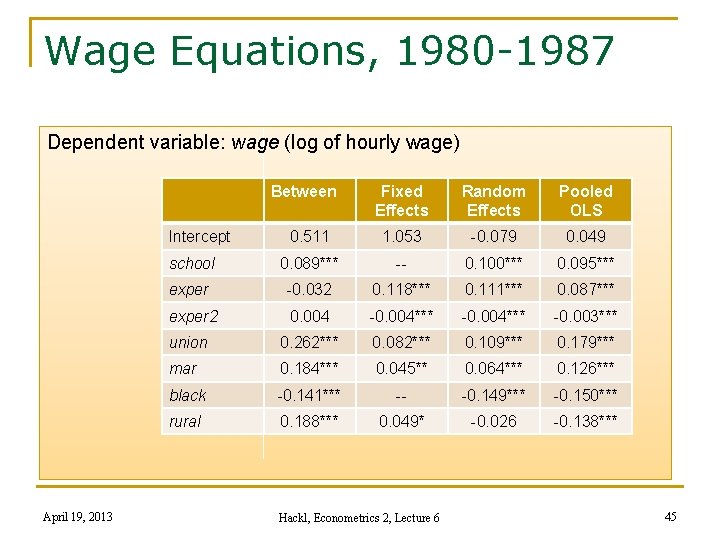
Wage Equations, 1980 -1987 Dependent variable: wage (log of hourly wage) Between Fixed Effects Random Effects Pooled OLS 0. 511 1. 053 -0. 079 0. 049 school 0. 089*** -- 0. 100*** 0. 095*** exper -0. 032 0. 118*** 0. 111*** 0. 087*** exper 2 0. 004 -0. 004*** -0. 003*** union 0. 262*** 0. 082*** 0. 109*** 0. 179*** mar 0. 184*** 0. 045** 0. 064*** 0. 126*** black -0. 141*** -- -0. 149*** -0. 150*** rural 0. 188*** 0. 049* -0. 026 -0. 138*** Intercept April 19, 2013 Hackl, Econometrics 2, Lecture 6 45

Contents n n n n Panel Data Pooling Independent Cross-sectional Data Panel Data: Pooled OLS Estimation Panel Data Models Fixed Effects Model Random Effects Model Analysis of Panel Data Models Panel Data in GRETL April 19, 2013 Hackl, Econometrics 2, Lecture 6 46

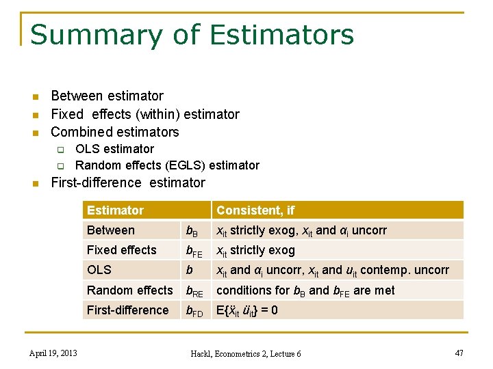
Summary of Estimators n n n Between estimator Fixed effects (within) estimator Combined estimators n OLS estimator Random effects (EGLS) estimator First-difference estimator Estimator April 19, 2013 Consistent, if Between b. B xit strictly exog, xit and αi uncorr Fixed effects b. FE xit strictly exog OLS b xit and αi uncorr, xit and uit contemp. uncorr Random effects b. RE conditions for b. B and b. FE are met First-difference E{ẍit üit} = 0 b. FD Hackl, Econometrics 2, Lecture 6 47

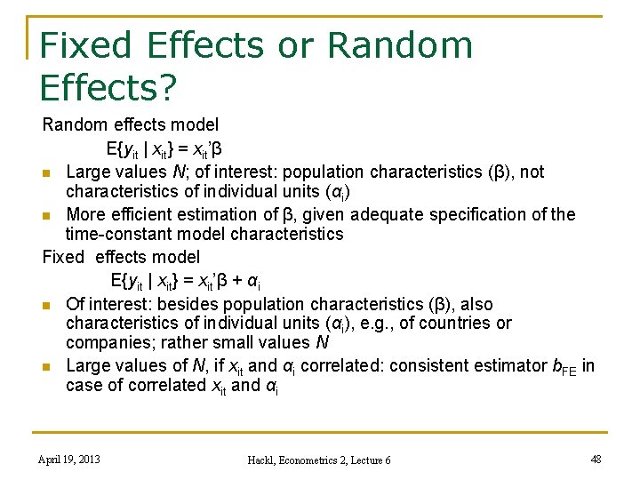
Fixed Effects or Random Effects? Random effects model E{yit | xit} = xit’β n Large values N; of interest: population characteristics (β), not characteristics of individual units (αi) n More efficient estimation of β, given adequate specification of the time-constant model characteristics Fixed effects model E{yit | xit} = xit’β + αi n Of interest: besides population characteristics (β), also characteristics of individual units (αi), e. g. , of countries or companies; rather small values N n Large values of N, if xit and αi correlated: consistent estimator b. FE in case of correlated xit and αi April 19, 2013 Hackl, Econometrics 2, Lecture 6 48

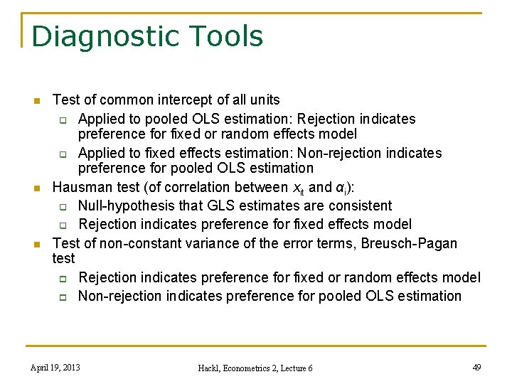
Diagnostic Tools n n n Test of common intercept of all units Applied to pooled OLS estimation: Rejection indicates preference for fixed or random effects model Applied to fixed effects estimation: Non-rejection indicates preference for pooled OLS estimation Hausman test (of correlation between xit and αi): Null-hypothesis that GLS estimates are consistent Rejection indicates preference for fixed effects model Test of non-constant variance of the error terms, Breusch-Pagan test Rejection indicates preference for fixed or random effects model Non-rejection indicates preference for pooled OLS estimation April 19, 2013 Hackl, Econometrics 2, Lecture 6 49

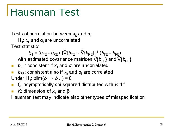
Hausman Tests of correlation between xit and αi H 0: xit and αi are uncorrelated Test statistic: ξH = (b. FE - b. RE)‘ [Ṽ{b. FE} - Ṽ{b. RE}]-1 (b. FE - b. RE) with estimated covariance matrices Ṽ{b. FE} and Ṽ{b. RE} n b. RE: consistent if xit and αi are uncorrelated n b. FE: consistent also if xit and αi are correlated Under H 0: plim(b. FE - b. RE) = 0 n ξH asymptotically chi-squared distributed with K d. f. n K: dimension of xit and β Hausman test may indicate also other types of misspecification April 19, 2013 Hackl, Econometrics 2, Lecture 6 50

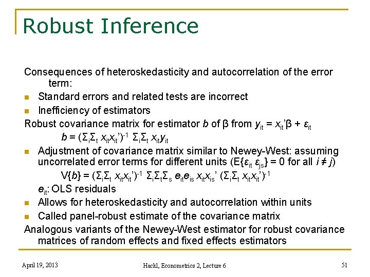
Robust Inference Consequences of heteroskedasticity and autocorrelation of the error term: n Standard errors and related tests are incorrect n Inefficiency of estimators Robust covariance matrix for estimator b of β from yit = xit’β + εit b = (ΣiΣt xitxit’)-1 ΣiΣt xityit n Adjustment of covariance matrix similar to Newey-West: assuming uncorrelated error terms for different units (E{εit εjs} = 0 for all i ≠ j) V{b} = (ΣiΣt xitxit’)-1 ΣiΣtΣs eiteis xitxis’ (ΣiΣt xitxit’)-1 eit: OLS residuals n Allows for heteroskedasticity and autocorrelation within units n Called panel-robust estimate of the covariance matrix Analogous variants of the Newey-West estimator for robust covariance matrices of random effects and fixed effects estimators April 19, 2013 Hackl, Econometrics 2, Lecture 6 51

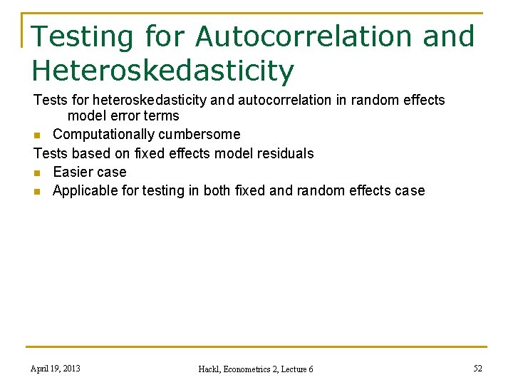
Testing for Autocorrelation and Heteroskedasticity Tests for heteroskedasticity and autocorrelation in random effects model error terms n Computationally cumbersome Tests based on fixed effects model residuals n Easier case n Applicable for testing in both fixed and random effects case April 19, 2013 Hackl, Econometrics 2, Lecture 6 52

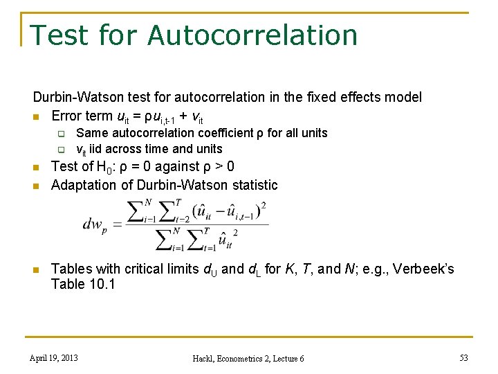
Test for Autocorrelation Durbin-Watson test for autocorrelation in the fixed effects model n Error term uit = ρui, t-1 + vit n n n Same autocorrelation coefficient ρ for all units vit iid across time and units Test of H 0: ρ = 0 against ρ > 0 Adaptation of Durbin-Watson statistic Tables with critical limits d. U and d. L for K, T, and N; e. g. , Verbeek’s Table 10. 1 April 19, 2013 Hackl, Econometrics 2, Lecture 6 53

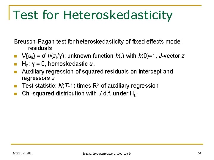
Test for Heteroskedasticity Breusch-Pagan test for heteroskedasticity of fixed effects model residuals n V{uit} = σ2 h(zit’γ); unknown function h(. ) with h(0)=1, J-vector z n H 0: γ = 0, homoskedastic uit n Auxiliary regression of squared residuals on intercept and regressors z n Test statistic: N(T-1) times R 2 of auxiliary regression n Chi-squared distribution with J d. f. under H 0 April 19, 2013 Hackl, Econometrics 2, Lecture 6 54

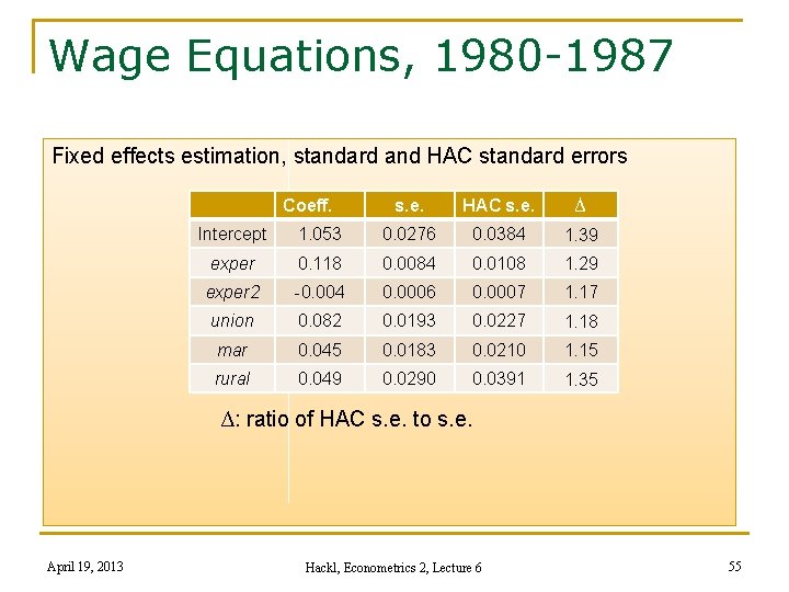
Wage Equations, 1980 -1987 Fixed effects estimation, standard and HAC standard errors Coeff. s. e. HAC s. e. ∆ Intercept 1. 053 0. 0276 0. 0384 1. 39 exper 0. 118 0. 0084 0. 0108 1. 29 exper 2 -0. 004 0. 0006 0. 0007 1. 17 union 0. 082 0. 0193 0. 0227 1. 18 mar 0. 045 0. 0183 0. 0210 1. 15 rural 0. 049 0. 0290 0. 0391 1. 35 ∆: ratio of HAC s. e. to s. e. April 19, 2013 Hackl, Econometrics 2, Lecture 6 55

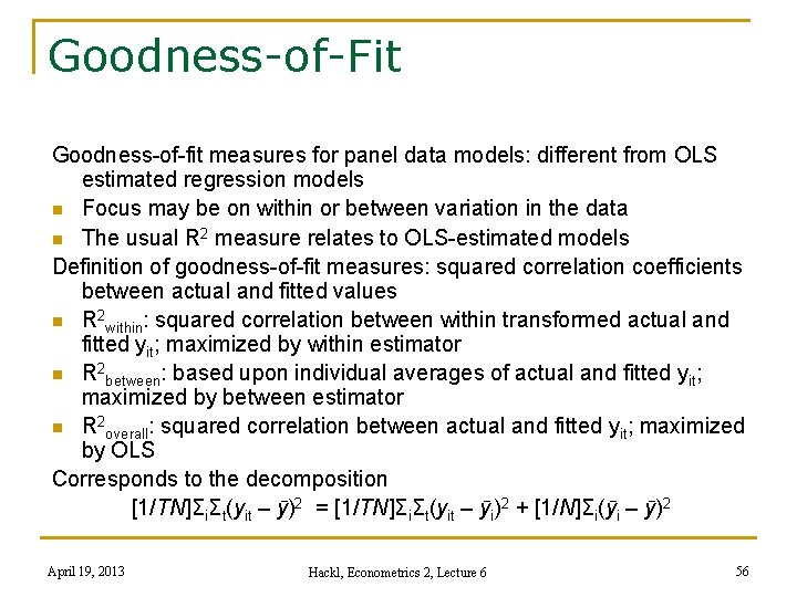
Goodness-of-Fit Goodness-of-fit measures for panel data models: different from OLS estimated regression models n Focus may be on within or between variation in the data n The usual R 2 measure relates to OLS-estimated models Definition of goodness-of-fit measures: squared correlation coefficients between actual and fitted values n R 2 within: squared correlation between within transformed actual and fitted yit; maximized by within estimator n R 2 between: based upon individual averages of actual and fitted yit; maximized by between estimator n R 2 overall: squared correlation between actual and fitted yit; maximized by OLS Corresponds to the decomposition [1/TN]ΣiΣt(yit – ӯ)2 = [1/TN]ΣiΣt(yit – ӯi)2 + [1/N]Σi(ӯi – ӯ)2 April 19, 2013 Hackl, Econometrics 2, Lecture 6 56

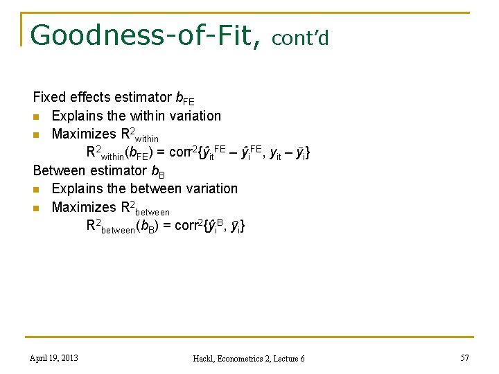
Goodness-of-Fit, cont’d Fixed effects estimator b. FE n Explains the within variation n Maximizes R 2 within(b. FE) = corr 2{ŷit. FE – ŷi. FE, yit – ӯi} Between estimator b. B n Explains the between variation n Maximizes R 2 between(b. B) = corr 2{ŷi. B, ӯi} April 19, 2013 Hackl, Econometrics 2, Lecture 6 57

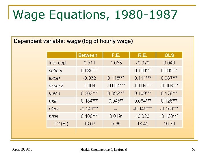
Wage Equations, 1980 -1987 Dependent variable: wage (log of hourly wage) Between F. E. R. E. OLS 0. 511 1. 053 -0. 079 0. 049 school 0. 089*** -- 0. 100*** 0. 095*** exper -0. 032 0. 118*** 0. 111*** 0. 087*** exper 2 0. 004 -0. 004*** -0. 003*** union 0. 262*** 0. 082*** 0. 109*** 0. 179*** mar 0. 184*** 0. 045** 0. 064*** 0. 126*** black -0. 141*** -- -0. 149*** -0. 150*** rural 0. 188*** 0. 049* -0. 026 -0. 138*** 16. 07 5. 66 18. 42 19. 70 Intercept R 2 (%) April 19, 2013 Hackl, Econometrics 2, Lecture 6 58

Contents n n n n Panel Data Pooling Independent Cross-sectional Data Panel Data: Pooled OLS Estimation Panel Data Models Fixed Effects Model Random Effects Model Analysis of Panel Data Models Panel Data in GRETL April 19, 2013 Hackl, Econometrics 2, Lecture 6 59

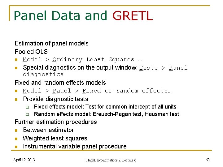
Panel Data and GRETL Estimation of panel models Pooled OLS n Model > Ordinary Least Squares … n Special diagnostics on the output window: Tests > Panel diagnostics Fixed and random effects models n Model > Panel > Fixed or random effects… n Provide diagnostic tests Fixed effects model: Test for common intercept of all units Random effects model: Breusch-Pagan test, Hausman test Further estimation procedures n Between estimator n Weighted least squares n Instrumental variable panel procedure April 19, 2013 Hackl, Econometrics 2, Lecture 6 60

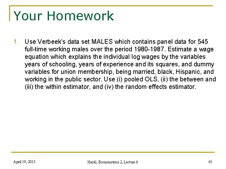
Your Homework 1. Use Verbeek’s data set MALES which contains panel data for 545 full-time working males over the period 1980 -1987. Estimate a wage equation which explains the individual log wages by the variables years of schooling, years of experience and its squares, and dummy variables for union membership, being married, black, Hispanic, and working in the public sector. Use (i) pooled OLS, (ii) the between and (iii) the within estimator, and (iv) the random effects estimator. April 19, 2013 Hackl, Econometrics 2, Lecture 6 61

Contents n n n n Panel Data Pooling Independent Cross-sectional Data Panel Data: Pooled OLS Estimation Panel Data Models Fixed Effects Model Random Effects Model Analysis of Panel Data Models Panel Data in GRETL April 19, 2013 Hackl, Econometrics 2, Lecture 6 62

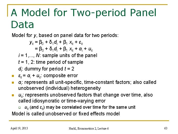
A Model for Two-period Panel Data Model for y, based on panel data for two periods: yit = β 0 + δ 1 dt + β 1 xit + εit = β 0 + δ 1 dt + β 1 xit + αi + uit i = 1, . . . , N: sample units of the panel t = 1, 2: time period of sample dt: dummy for period t = 2 n εit = αi + uit: composite error n αi: represents all unit-specific, time-constant factors; also called unobserved (individual) heterogeneity n uit: represents unobserved factors that change over time, also called idiosyncratic or time-varying error uit (and εit) may be correlated over time for the same unit Model is called unobserved or fixed effects model April 19, 2013 Hackl, Econometrics 2, Lecture 6 63

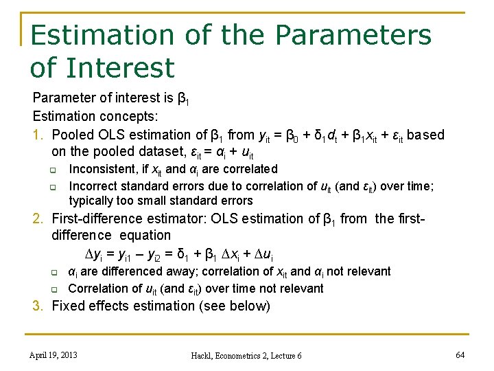
Estimation of the Parameters of Interest Parameter of interest is β 1 Estimation concepts: 1. Pooled OLS estimation of β 1 from yit = β 0 + δ 1 dt + β 1 xit + εit based on the pooled dataset, εit = αi + uit Inconsistent, if xit and αi are correlated Incorrect standard errors due to correlation of uit (and εit) over time; typically too small standard errors 2. First-difference estimator: OLS estimation of β 1 from the firstdifference equation ∆yi = yi 1 – yi 2 = δ 1 + β 1 ∆xi + ∆ui αi are differenced away; correlation of xit and αi not relevant Correlation of uit (and εit) over time not relevant 3. Fixed effects estimation (see below) April 19, 2013 Hackl, Econometrics 2, Lecture 6 64

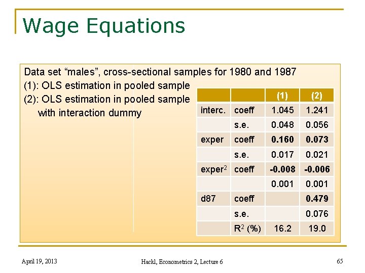
Wage Equations Data set “males”, cross-sectional samples for 1980 and 1987 (1): OLS estimation in pooled sample (1) (2): OLS estimation in pooled sample interc. coeff 1. 045 1. 241 with interaction dummy exper s. e. 0. 048 0. 056 coeff 0. 160 0. 073 s. e. 0. 017 0. 021 exper 2 coeff -0. 008 -0. 006 0. 001 d 87 coeff 0. 479 s. e. 0. 076 R 2 (%) April 19, 2013 Hackl, Econometrics 2, Lecture 6 0. 001 16. 2 19. 0 65

Pooled OLS Estimation Model for y, based on panel data from T periods: yit = xit‘β + εit Pooled OLS estimation of β n Assumes equal unit means αi n Consistent if xit and εit (at least contemporaneously) uncorrelated n Diagnostics of interest: Test whether panel data structure to be taken into account Test whether fixed or random effects model preferable In GRETL: output window of OLS estimation applied to panel data structure offers a special test: Test > Panel diagnostics n Tests H 0: pooled model preferable to fixed effects and random effects model n Hausman test (H 0: random effects model preferable to fixed effects model) April 19, 2013 Hackl, Econometrics 2, Lecture 6 66