Econometrics 2 Lecture 5 Multiequation Models Contents n

Econometrics 2 - Lecture 5 Multi-equation Models

Contents n n n Systems of Equations VAR Models Simultaneous Equations and VAR Models and Cointegration VEC Model: Cointegration Tests VEC Model: Specification and Estimation April 9, 2013 Hackl, Econometrics 2, Lecture 5 2

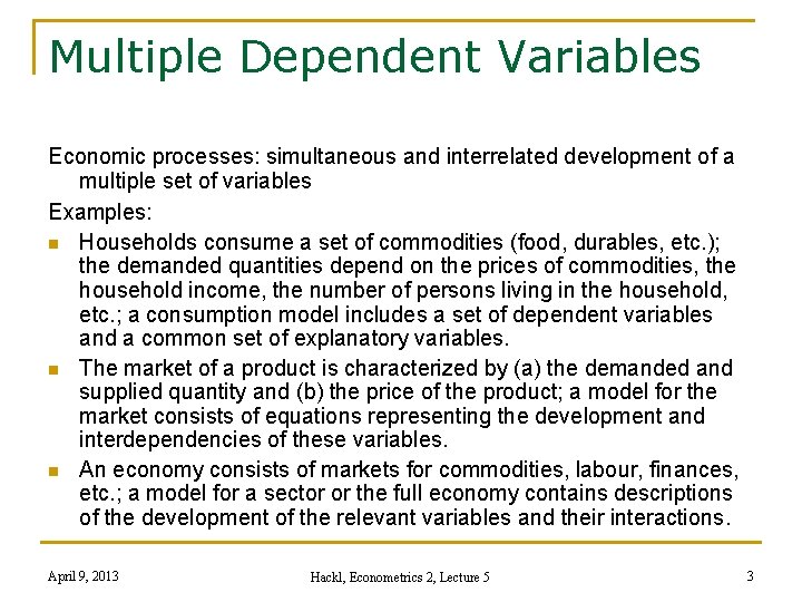
Multiple Dependent Variables Economic processes: simultaneous and interrelated development of a multiple set of variables Examples: n Households consume a set of commodities (food, durables, etc. ); the demanded quantities depend on the prices of commodities, the household income, the number of persons living in the household, etc. ; a consumption model includes a set of dependent variables and a common set of explanatory variables. n The market of a product is characterized by (a) the demanded and supplied quantity and (b) the price of the product; a model for the market consists of equations representing the development and interdependencies of these variables. n An economy consists of markets for commodities, labour, finances, etc. ; a model for a sector or the full economy contains descriptions of the development of the relevant variables and their interactions. April 9, 2013 Hackl, Econometrics 2, Lecture 5 3

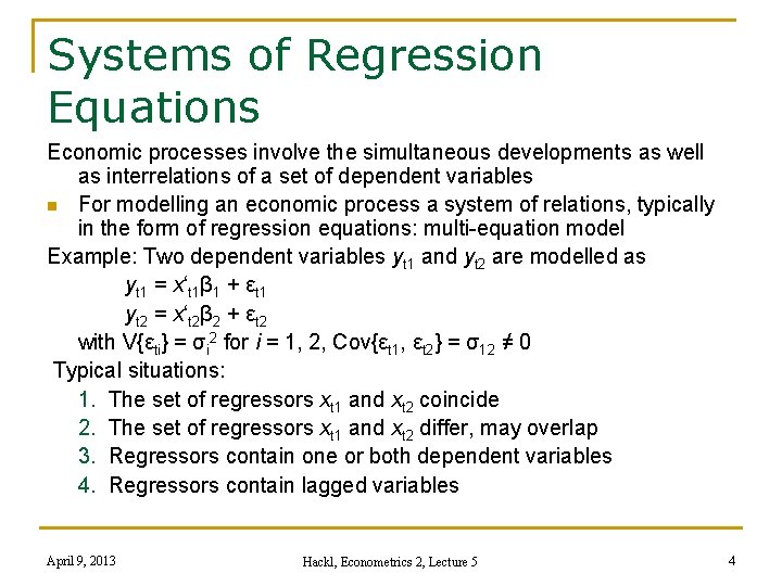
Systems of Regression Equations Economic processes involve the simultaneous developments as well as interrelations of a set of dependent variables n For modelling an economic process a system of relations, typically in the form of regression equations: multi-equation model Example: Two dependent variables yt 1 and yt 2 are modelled as yt 1 = x‘t 1β 1 + εt 1 yt 2 = x‘t 2β 2 + εt 2 with V{εti} = σi 2 for i = 1, 2, Cov{εt 1, εt 2} = σ12 ≠ 0 Typical situations: 1. The set of regressors xt 1 and xt 2 coincide 2. The set of regressors xt 1 and xt 2 differ, may overlap 3. Regressors contain one or both dependent variables 4. Regressors contain lagged variables April 9, 2013 Hackl, Econometrics 2, Lecture 5 4

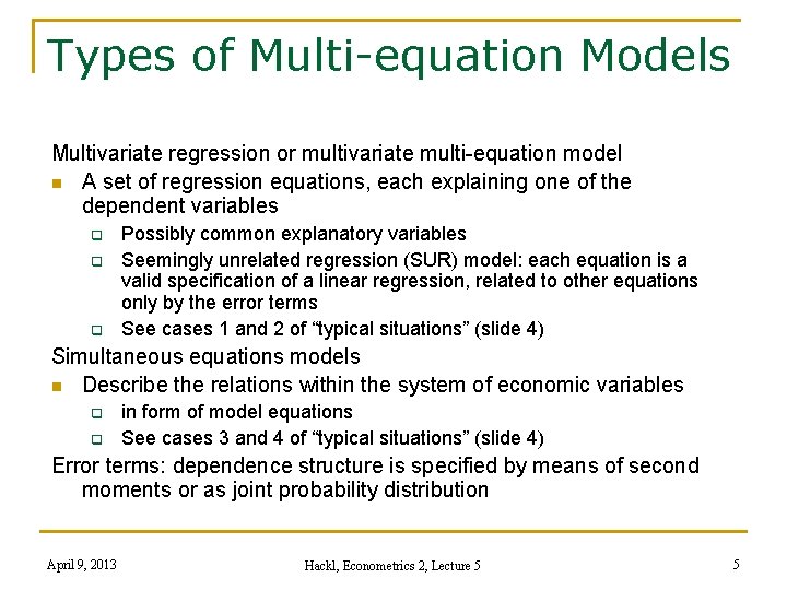
Types of Multi-equation Models Multivariate regression or multivariate multi-equation model n A set of regression equations, each explaining one of the dependent variables q q q Possibly common explanatory variables Seemingly unrelated regression (SUR) model: each equation is a valid specification of a linear regression, related to other equations only by the error terms See cases 1 and 2 of “typical situations” (slide 4) Simultaneous equations models n Describe the relations within the system of economic variables q q in form of model equations See cases 3 and 4 of “typical situations” (slide 4) Error terms: dependence structure is specified by means of second moments or as joint probability distribution April 9, 2013 Hackl, Econometrics 2, Lecture 5 5

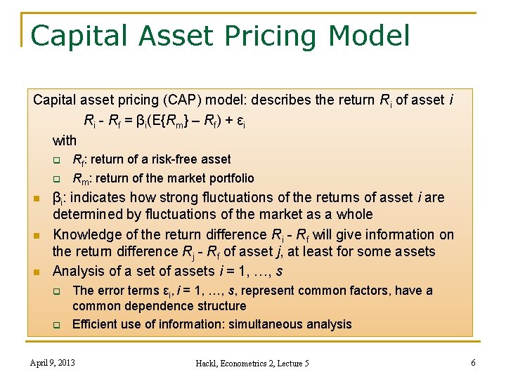
Capital Asset Pricing Model Capital asset pricing (CAP) model: describes the return Ri of asset i Ri - Rf = βi(E{Rm} – Rf) + εi with q q n n n Rf: return of a risk-free asset Rm: return of the market portfolio βi: indicates how strong fluctuations of the returns of asset i are determined by fluctuations of the market as a whole Knowledge of the return difference Ri - Rf will give information on the return difference Rj - Rf of asset j, at least for some assets Analysis of a set of assets i = 1, …, s q q The error terms εi, i = 1, …, s, represent common factors, have a common dependence structure Efficient use of information: simultaneous analysis April 9, 2013 Hackl, Econometrics 2, Lecture 5 6

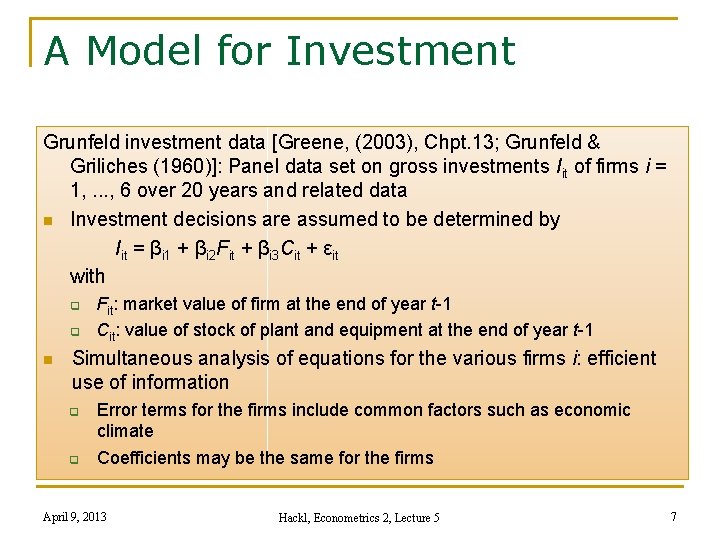
A Model for Investment Grunfeld investment data [Greene, (2003), Chpt. 13; Grunfeld & Griliches (1960)]: Panel data set on gross investments Iit of firms i = 1, . . . , 6 over 20 years and related data n Investment decisions are assumed to be determined by Iit = βi 1 + βi 2 Fit + βi 3 Cit + εit with q q n Fit: market value of firm at the end of year t-1 Cit: value of stock of plant and equipment at the end of year t-1 Simultaneous analysis of equations for the various firms i: efficient use of information q q Error terms for the firms include common factors such as economic climate Coefficients may be the same for the firms April 9, 2013 Hackl, Econometrics 2, Lecture 5 7

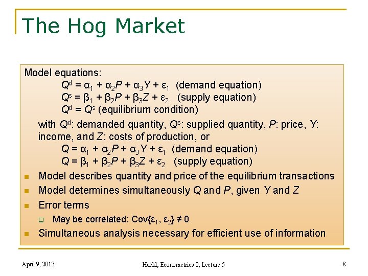
The Hog Market Model equations: Qd = α 1 + α 2 P + α 3 Y + ε 1 (demand equation) Qs = β 1 + β 2 P + β 3 Z + ε 2 (supply equation) Qd = Qs (equilibrium condition) with Qd: demanded quantity, Qs: supplied quantity, P: price, Y: income, and Z: costs of production, or Q = α 1 + α 2 P + α 3 Y + ε 1 (demand equation) Q = β 1 + β 2 P + β 3 Z + ε 2 (supply equation) n Model describes quantity and price of the equilibrium transactions n Model determines simultaneously Q and P, given Y and Z n Error terms q n May be correlated: Cov{ε 1, ε 2} ≠ 0 Simultaneous analysis necessary for efficient use of information April 9, 2013 Hackl, Econometrics 2, Lecture 5 8

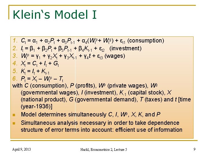
Klein‘s Model I 1. Ct = α 1 + α 2 Pt + α 3 Pt-1 + α 4(Wtp+ Wtg) + εt 1 (consumption) 2. It = β 1 + β 2 Pt + β 3 Pt-1 + β 4 Kt-1 + εt 2 (investment) 3. Wtp = γ 1 + γ 2 Xt + γ 3 Xt-1 + γ 4 t + εt 3 (wages) 4. Xt = Ct + It + Gt 5. Kt = It + Kt-1 6. Pt = Xt – Wtp – Tt with C (consumption), P (profits), Wp (private wages), Wg (governmental wages), I (investment), K-1 (capital stock), X (national product), G (governmental demand), T (taxes) and t [time (year-1936)] n Model determines simultaneously C, I, Wp, X, K, and P n Simultaneous analysis necessary in order to take dependence structure of error terms into account: efficient use of information April 9, 2013 Hackl, Econometrics 2, Lecture 5 9

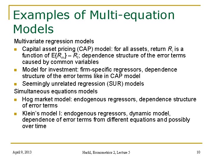
Examples of Multi-equation Models Multivariate regression models n Capital asset pricing (CAP) model: for all assets, return Ri is a function of E{Rm} – Rf; dependence structure of the error terms caused by common variables n Model for investment: firm-specific regressors, dependence structure of the error terms like in CAP model n Seemingly unrelated regression (SUR) models Simultaneous equations models n Hog market model: endogenous regressors, dependence structure of error terms n Klein’s model I: endogenous regressors, dynamic model, dependence of error terms from different equations and possibly over time April 9, 2013 Hackl, Econometrics 2, Lecture 5 10

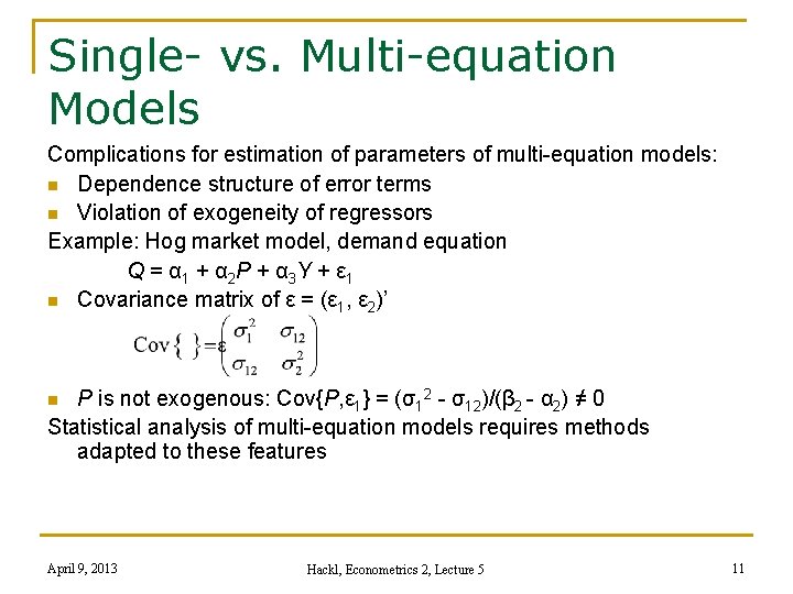
Single- vs. Multi-equation Models Complications for estimation of parameters of multi-equation models: n Dependence structure of error terms n Violation of exogeneity of regressors Example: Hog market model, demand equation Q = α 1 + α 2 P + α 3 Y + ε 1 n Covariance matrix of ε = (ε 1, ε 2)’ P is not exogenous: Cov{P, ε 1} = (σ12 - σ12)/(β 2 - α 2) ≠ 0 Statistical analysis of multi-equation models requires methods adapted to these features n April 9, 2013 Hackl, Econometrics 2, Lecture 5 11

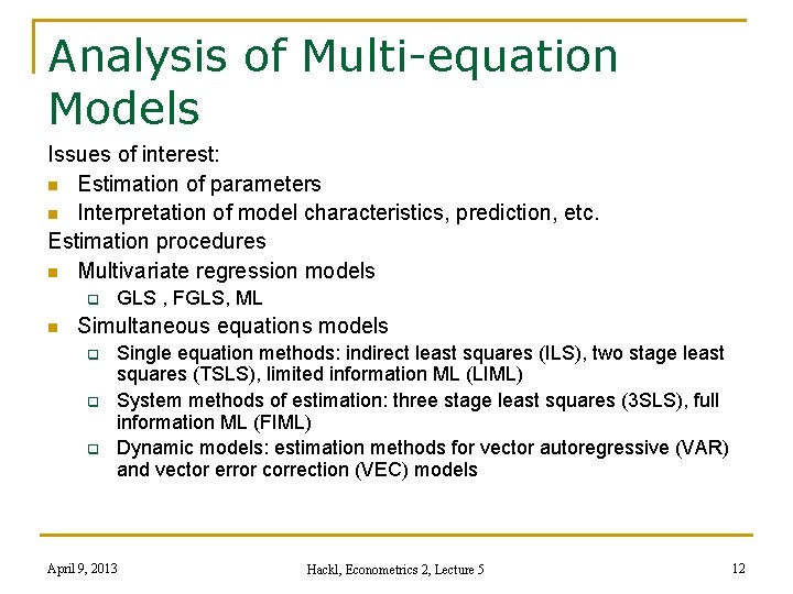
Analysis of Multi-equation Models Issues of interest: n Estimation of parameters n Interpretation of model characteristics, prediction, etc. Estimation procedures n Multivariate regression models q n GLS , FGLS, ML Simultaneous equations models q q q Single equation methods: indirect least squares (ILS), two stage least squares (TSLS), limited information ML (LIML) System methods of estimation: three stage least squares (3 SLS), full information ML (FIML) Dynamic models: estimation methods for vector autoregressive (VAR) and vector error correction (VEC) models April 9, 2013 Hackl, Econometrics 2, Lecture 5 12

Contents n n n Systems of Equations VAR Models Simultaneous Equations and VAR Models and Cointegration VEC Model: Cointegration Tests VEC Model: Specification and Estimation April 9, 2013 Hackl, Econometrics 2, Lecture 5 13

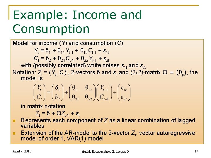
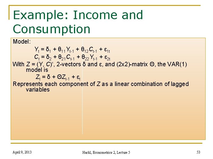
Example: Income and Consumption Model for income (Y) and consumption (C) Yt = δ 1 + θ 11 Yt-1 + θ 12 Ct-1 + ε 1 t Ct = δ 2 + θ 21 Ct-1 + θ 22 Yt-1 + ε 2 t with (possibly correlated) white noises ε 1 t and ε 2 t Notation: Zt = (Yt, Ct)‘, 2 -vectors δ and ε, and (2 x 2)-matrix Θ = (θij), the model is n n in matrix notation Zt = δ + ΘZt-1 + εt Represents each component of Z as a linear combination of lagged variables Extension of the AR-model to the 2 -vector Zt: vector autoregressive model of order 1, VAR(1) model April 9, 2013 Hackl, Econometrics 2, Lecture 5 14

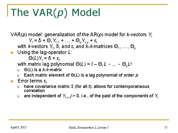
The VAR(p) Model VAR(p) model: generalization of the AR(p) model for k-vectors Yt Yt = δ + Θ 1 Yt-1 + … + Θp. Yt-p + εt with k-vectors Yt, δ, and εt and kxk-matrices Θ 1, …, Θp n Using the lag-operator L: Θ(L)Yt = δ + εt with matrix lag polynomial Θ(L) = I – Θ 1 L - … - Θp. Lp q q n Θ(L) is a kxk-matrix Each matrix element of Θ(L) is a lag polynomial of order p Error terms εt q q have covariance matrix Σ (for all t); allows for contemporaneous correlation are independent of Yt-j, j > 0, i. e. , of the past of the components of Yt April 9, 2013 Hackl, Econometrics 2, Lecture 5 15

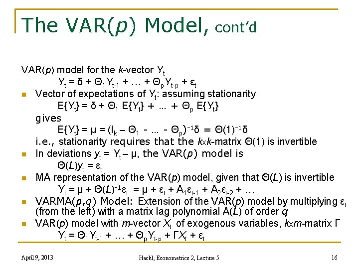
The VAR(p) Model, cont’d VAR(p) model for the k-vector Yt Yt = δ + Θ 1 Yt-1 + … + Θp. Yt-p + εt n Vector of expectations of Yt: assuming stationarity E{Yt} = δ + Θ 1 E{Yt} + … + Θp E{Yt} gives E{Yt} = μ = (Ik – Θ 1 - … - Θp)-1δ = Θ(1)-1δ i. e. , stationarity requires that the kxk-matrix Θ(1) is invertible n In deviations yt = Yt – μ, the VAR(p) model is Θ(L)yt = εt n MA representation of the VAR(p) model, given that Θ(L) is invertible Yt = μ + Θ(L)-1εt = μ + εt + A 1εt-1 + A 2εt-2 + … n VARMA(p, q) Model: Extension of the VAR(p) model by multiplying εt (from the left) with a matrix lag polynomial A(L) of order q n VAR(p) model with m-vector Xt of exogenous variables, kxm-matrix Γ Yt = Θ 1 Yt-1 + … + Θp. Yt-p + ΓXt + εt April 9, 2013 Hackl, Econometrics 2, Lecture 5 16

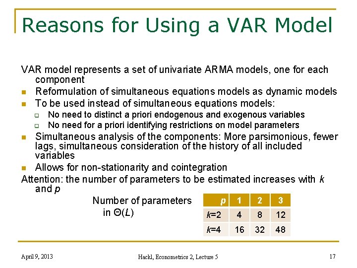
Reasons for Using a VAR Model VAR model represents a set of univariate ARMA models, one for each component n Reformulation of simultaneous equations models as dynamic models n To be used instead of simultaneous equations models: q q No need to distinct a priori endogenous and exogenous variables No need for a priori identifying restrictions on model parameters Simultaneous analysis of the components: More parsimonious, fewer lags, simultaneous consideration of the history of all included variables n Allows for non-stationarity and cointegration Attention: the number of parameters to be estimated increases with k and p p 1 2 3 Number of parameters in Θ(L) k=2 4 8 12 n k=4 April 9, 2013 Hackl, Econometrics 2, Lecture 5 16 32 48 17

Contents n n n Systems of Equations VAR Models Simultaneous Equations and VAR Models and Cointegration VEC Model: Cointegration Tests VEC Model: Specification and Estimation April 9, 2013 Hackl, Econometrics 2, Lecture 5 18

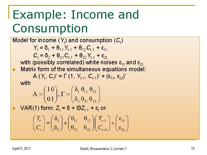
Example: Income and Consumption Model for income (Yt) and consumption (Ct) Yt = δ 1 + θ 11 Yt-1 + θ 12 Ct-1 + ε 1 t Ct = δ 2 + θ 21 Ct-1 + θ 22 Yt-1 + ε 2 t with (possibly correlated) white noises ε 1 t and ε 2 t n Matrix form of the simultaneous equations model: A (Yt, Ct)‘ = Γ (1, Yt-1, Ct-1)‘ + (ε 1 t, ε 2 t)’ with n VAR(1) form: Zt = δ + ΘZt-1 + εt or April 9, 2013 Hackl, Econometrics 2, Lecture 5 19

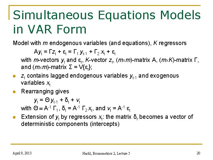
Simultaneous Equations Models in VAR Form Model with m endogenous variables (and equations), K regressors Ayt = Γzt + εt = Γ 1 yt-1 + Γ 2 xt + εt with m-vectors yt and εt, K-vector zt, (mxm)-matrix A, (mx. K)-matrix Γ, and (mxm)-matrix Σ = V{εt}; n zt contains lagged endogenous variables yt-1 and exogenous variables xt n Rearranging gives yt = Θ yt-1 + δt + vt with Θ = A-1 Γ 1, δt = A-1 Γ 2 xt, and vt = A-1 εt n Extension of yt by regressors xt: the matrix δt becomes a vector of deterministic components (intercepts) April 9, 2013 Hackl, Econometrics 2, Lecture 5 20

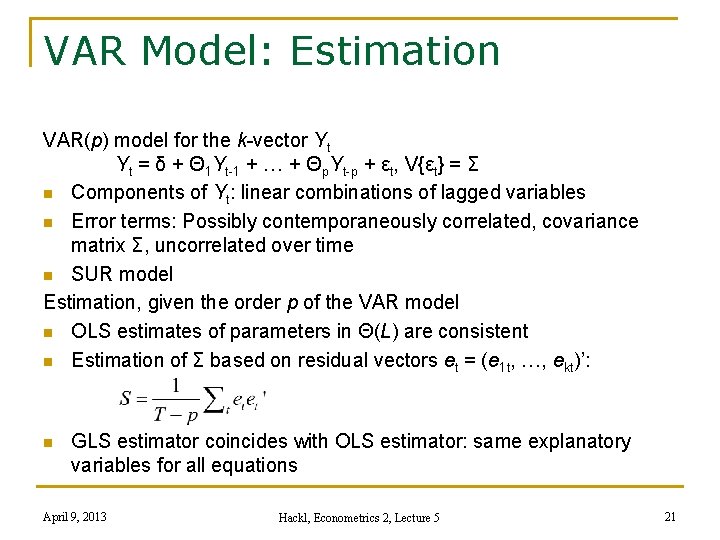
VAR Model: Estimation VAR(p) model for the k-vector Yt Yt = δ + Θ 1 Yt-1 + … + Θp. Yt-p + εt, V{εt} = Σ n Components of Yt: linear combinations of lagged variables n Error terms: Possibly contemporaneously correlated, covariance matrix Σ, uncorrelated over time n SUR model Estimation, given the order p of the VAR model n OLS estimates of parameters in Θ(L) are consistent n Estimation of Σ based on residual vectors et = (e 1 t, …, ekt)’: n GLS estimator coincides with OLS estimator: same explanatory variables for all equations April 9, 2013 Hackl, Econometrics 2, Lecture 5 21

VAR Model: Estimation, cont’d Choice of the order p of the VAR model n Estimation of VAR models for various orders p n Choice of p based on Akaike or Schwarz information criterion April 9, 2013 Hackl, Econometrics 2, Lecture 5 22

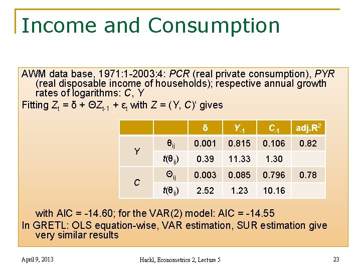
Income and Consumption AWM data base, 1971: 1 -2003: 4: PCR (real private consumption), PYR (real disposable income of households); respective annual growth rates of logarithms: C, Y Fitting Zt = δ + ΘZt-1 + εt with Z = (Y, C)‘ gives Y C δ Y-1 C-1 adj. R 2 θij 0. 001 0. 815 0. 106 0. 82 t(θij) 0. 39 11. 33 1. 30 Θij 0. 003 0. 085 0. 796 t(θij) 2. 52 1. 23 10. 16 0. 78 with AIC = -14. 60; for the VAR(2) model: AIC = -14. 55 In GRETL: OLS equation-wise, VAR estimation, SUR estimation give very similar results April 9, 2013 Hackl, Econometrics 2, Lecture 5 23

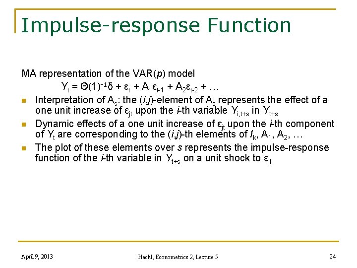
Impulse-response Function MA representation of the VAR(p) model Yt = Θ(1)-1δ + εt + A 1εt-1 + A 2εt-2 + … n Interpretation of As: the (i, j)-element of As represents the effect of a one unit increase of εjt upon the i-th variable Yi, t+s in Yt+s n Dynamic effects of a one unit increase of εjt upon the i-th component of Yt are corresponding to the (i, j)-th elements of Ik, A 1, A 2, … n The plot of these elements over s represents the impulse-response function of the i-th variable in Yt+s on a unit shock to εjt April 9, 2013 Hackl, Econometrics 2, Lecture 5 24

Contents n n n Systems of Equations VAR Models Simultaneous Equations and VAR Models and Cointegration VEC Model: Cointegration Tests VEC Model: Specification and Estimation April 9, 2013 Hackl, Econometrics 2, Lecture 5 25

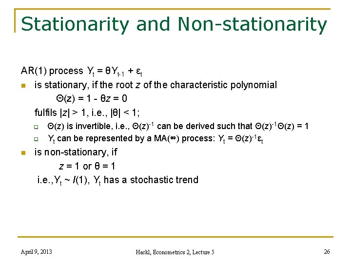
Stationarity and Non-stationarity AR(1) process Yt = θYt-1 + εt n is stationary, if the root z of the characteristic polynomial Θ(z) = 1 - θz = 0 fulfils |z| > 1, i. e. , |θ| < 1; q q n Θ(z) is invertible, i. e. , Θ(z)-1 can be derived such that Θ(z)-1Θ(z) = 1 Yt can be represented by a MA(∞) process: Yt = Θ(z)-1εt is non-stationary, if z = 1 or θ = 1 i. e. , Yt ~ I(1), Yt has a stochastic trend April 9, 2013 Hackl, Econometrics 2, Lecture 5 26

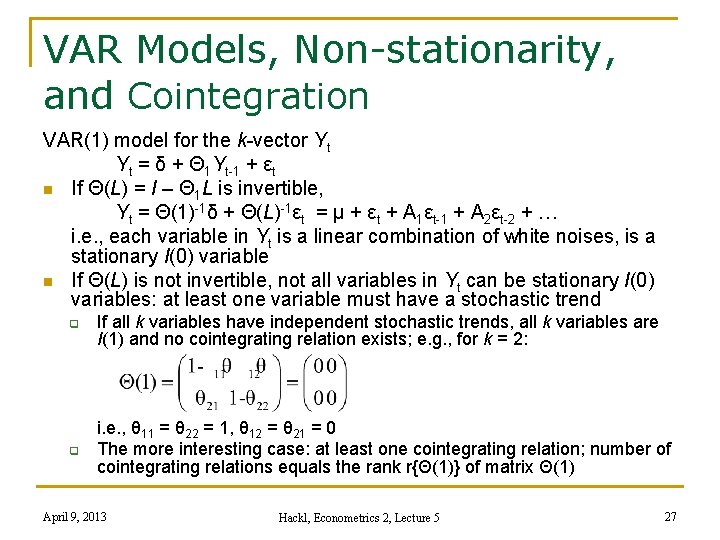
VAR Models, Non-stationarity, and Cointegration VAR(1) model for the k-vector Yt Yt = δ + Θ 1 Yt-1 + εt n If Θ(L) = I – Θ 1 L is invertible, Yt = Θ(1)-1δ + Θ(L)-1εt = μ + εt + A 1εt-1 + A 2εt-2 + … i. e. , each variable in Yt is a linear combination of white noises, is a stationary I(0) variable n If Θ(L) is not invertible, not all variables in Yt can be stationary I(0) variables: at least one variable must have a stochastic trend q q If all k variables have independent stochastic trends, all k variables are I(1) and no cointegrating relation exists; e. g. , for k = 2: i. e. , θ 11 = θ 22 = 1, θ 12 = θ 21 = 0 The more interesting case: at least one cointegrating relation; number of cointegrating relations equals the rank r{Θ(1)} of matrix Θ(1) April 9, 2013 Hackl, Econometrics 2, Lecture 5 27

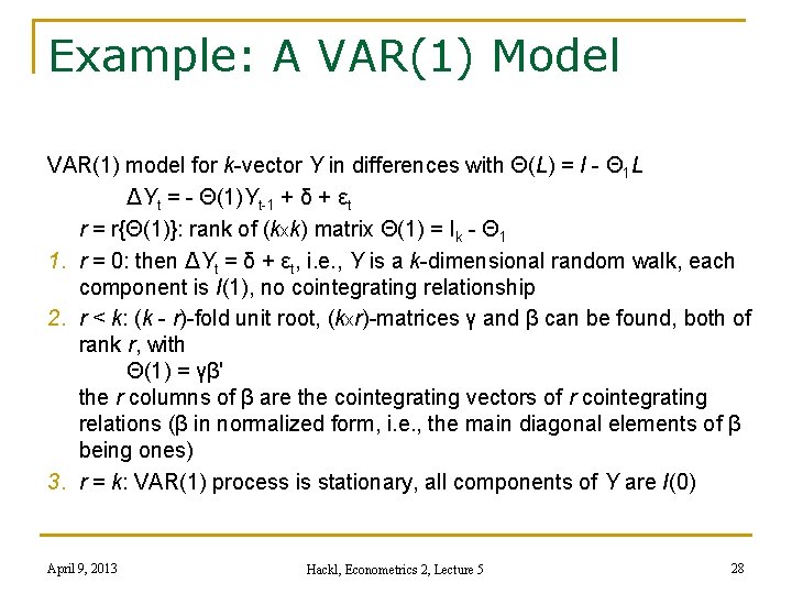
Example: A VAR(1) Model VAR(1) model for k-vector Y in differences with Θ(L) = I - Θ 1 L ΔYt = - Θ(1)Yt-1 + δ + εt r = r{Θ(1)}: rank of (kxk) matrix Θ(1) = Ik - Θ 1 1. r = 0: then ΔYt = δ + εt, i. e. , Y is a k-dimensional random walk, each component is I(1), no cointegrating relationship 2. r < k: (k - r)-fold unit root, (kxr)-matrices γ and β can be found, both of rank r, with Θ(1) = γβ' the r columns of β are the cointegrating vectors of r cointegrating relations (β in normalized form, i. e. , the main diagonal elements of β being ones) 3. r = k: VAR(1) process is stationary, all components of Y are I(0) April 9, 2013 Hackl, Econometrics 2, Lecture 5 28

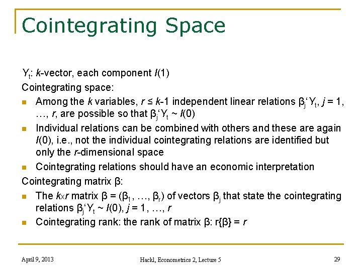
Cointegrating Space Yt: k-vector, each component I(1) Cointegrating space: n Among the k variables, r ≤ k-1 independent linear relations βj‘Yt, j = 1, …, r, are possible so that βj‘Yt ~ I(0) n Individual relations can be combined with others and these are again I(0), i. e. , not the individual cointegrating relations are identified but only the r-dimensional space n Cointegrating relations should have an economic interpretation Cointegrating matrix β: n The kxr matrix β = (β 1, …, βr) of vectors βj that state the cointegrating relations βj‘Yt ~ I(0), j = 1, …, r n Cointegrating rank: the rank of matrix β: r{β} = r April 9, 2013 Hackl, Econometrics 2, Lecture 5 29

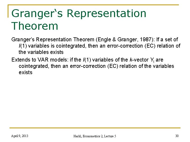
Granger‘s Representation Theorem Granger’s Representation Theorem (Engle & Granger, 1987): If a set of I(1) variables is cointegrated, then an error-correction (EC) relation of the variables exists Extends to VAR models: if the I(1) variables of the k-vector Yt are cointegrated, then an error-correction (EC) relation of the variables exists April 9, 2013 Hackl, Econometrics 2, Lecture 5 30

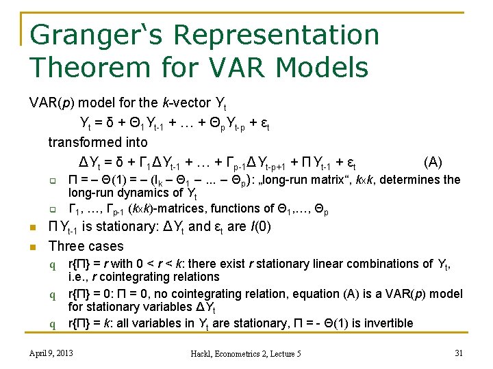
Granger‘s Representation Theorem for VAR Models VAR(p) model for the k-vector Yt Yt = δ + Θ 1 Yt-1 + … + Θp. Yt-p + εt transformed into ΔYt = δ + Γ 1ΔYt-1 + … + Γp-1ΔYt-p+1 + ΠYt-1 + εt q q n n (A) Π = – Θ(1) = – (Ik – Θ 1 – … – Θp): „long-run matrix“, kxk, determines the long-run dynamics of Yt Γ 1, …, Γp-1 (kxk)-matrices, functions of Θ 1, …, Θp ΠYt-1 is stationary: ΔYt and εt are I(0) Three cases q q q r{Π} = r with 0 < r < k: there exist r stationary linear combinations of Yt, i. e. , r cointegrating relations r{Π} = 0: Π = 0, no cointegrating relation, equation (A) is a VAR(p) model for stationary variables ΔYt r{Π} = k: all variables in Yt are stationary, Π = - Θ(1) is invertible April 9, 2013 Hackl, Econometrics 2, Lecture 5 31

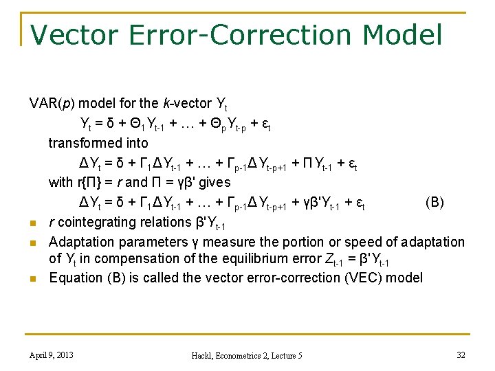
Vector Error-Correction Model VAR(p) model for the k-vector Yt Yt = δ + Θ 1 Yt-1 + … + Θp. Yt-p + εt transformed into ΔYt = δ + Γ 1ΔYt-1 + … + Γp-1ΔYt-p+1 + ΠYt-1 + εt with r{Π} = r and Π = γβ' gives ΔYt = δ + Γ 1ΔYt-1 + … + Γp-1ΔYt-p+1 + γβ'Yt-1 + εt (B) n r cointegrating relations β'Yt-1 n Adaptation parameters γ measure the portion or speed of adaptation of Yt in compensation of the equilibrium error Zt-1 = β'Yt-1 n Equation (B) is called the vector error-correction (VEC) model April 9, 2013 Hackl, Econometrics 2, Lecture 5 32

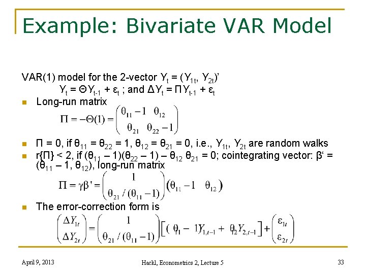
Example: Bivariate VAR Model VAR(1) model for the 2 -vector Yt = (Y 1 t, Y 2 t)’ Yt = ΘYt-1 + εt ; and ΔYt = ΠYt-1 + εt n Long-run matrix n Π = 0, if θ 11 = θ 22 = 1, θ 12 = θ 21 = 0, i. e. , Y 1 t, Y 2 t are random walks r{Π} < 2, if (θ 11 – 1)(θ 22 – 1) – θ 12 θ 21 = 0; cointegrating vector: β‘ = (θ 11 – 1, θ 12), long-run matrix n The error-correction form is n April 9, 2013 Hackl, Econometrics 2, Lecture 5 33

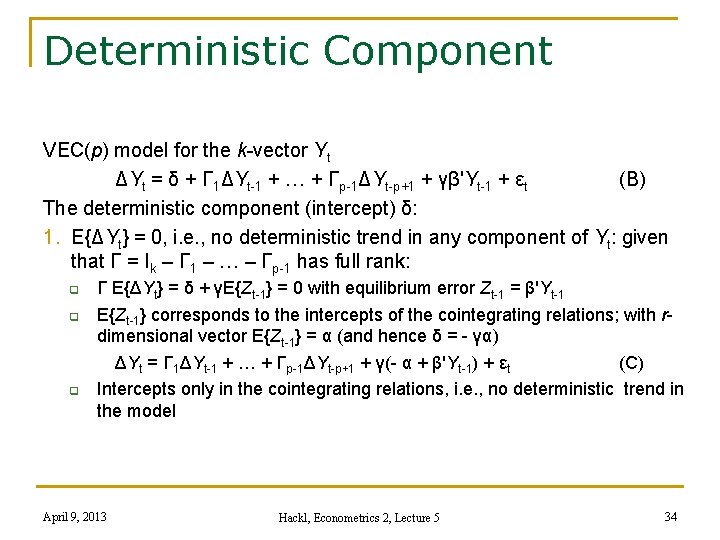
Deterministic Component VEC(p) model for the k-vector Yt ΔYt = δ + Γ 1ΔYt-1 + … + Γp-1ΔYt-p+1 + γβ'Yt-1 + εt (B) The deterministic component (intercept) δ: 1. E{ΔYt} = 0, i. e. , no deterministic trend in any component of Yt: given that Γ = Ik – Γ 1 – … – Γp-1 has full rank: q q q Γ E{ΔYt} = δ + γE{Zt-1} = 0 with equilibrium error Zt-1 = β'Yt-1 E{Zt-1} corresponds to the intercepts of the cointegrating relations; with rdimensional vector E{Zt-1} = α (and hence δ = - γα) ΔYt = Γ 1ΔYt-1 + … + Γp-1ΔYt-p+1 + γ(- α + β'Yt-1) + εt (C) Intercepts only in the cointegrating relations, i. e. , no deterministic trend in the model April 9, 2013 Hackl, Econometrics 2, Lecture 5 34

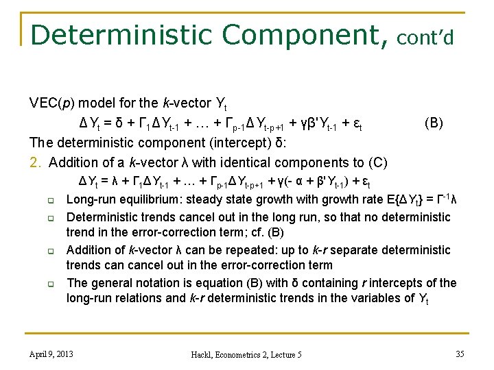
Deterministic Component, cont’d VEC(p) model for the k-vector Yt ΔYt = δ + Γ 1ΔYt-1 + … + Γp-1ΔYt-p+1 + γβ'Yt-1 + εt The deterministic component (intercept) δ: 2. Addition of a k-vector λ with identical components to (C) q q (B) ΔYt = λ + Γ 1ΔYt-1 + … + Γp-1ΔYt-p+1 + γ(- α + β'Yt-1) + εt Long-run equilibrium: steady state growth with growth rate E{ΔYt} = Γ-1λ Deterministic trends cancel out in the long run, so that no deterministic trend in the error-correction term; cf. (B) Addition of k-vector λ can be repeated: up to k-r separate deterministic trends cancel out in the error-correction term The general notation is equation (B) with δ containing r intercepts of the long-run relations and k-r deterministic trends in the variables of Yt April 9, 2013 Hackl, Econometrics 2, Lecture 5 35

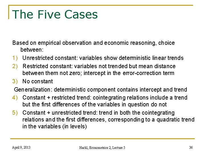
The Five Cases Based on empirical observation and economic reasoning, choice between: 1) Unrestricted constant: variables show deterministic linear trends 2) Restricted constant: variables not trended but mean distance between them not zero; intercept in the error-correction term 3) No constant Generalization: deterministic component contains intercept and trend 4) Constant + restricted trend: cointegrating relations include a trend but the first differences of the variables in question do not 5) Constant + unrestricted trend: trend in both the cointegrating relations and the first differences, corresponding to a quadratic trend in the variables (in levels) April 9, 2013 Hackl, Econometrics 2, Lecture 5 36

Contents n n n Systems of Equations VAR Models Simultaneous Equations and VAR Models and Cointegration VEC Model: Cointegration Tests VEC Model: Specification and Estimation April 9, 2013 Hackl, Econometrics 2, Lecture 5 37

Choice of the Cointegrating Rank Based on k-vector Yt ~ I(1) Estimation procedure needs as input the cointegrating rank r Testing for cointegration n Engle-Granger approach n Johansen‘s R 3 method April 9, 2013 Hackl, Econometrics 2, Lecture 5 38

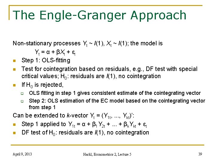
The Engle-Granger Approach Non-stationary processes Yt ~ I(1), Xt ~ I(1); the model is Yt = α + βXt + εt n Step 1: OLS-fitting n Test for cointegration based on residuals, e. g. , DF test with special critical values; H 0: residuals are I(1), no cointegration n If H 0 is rejected, q q OLS fitting in step 1 gives consistent estimate of the cointegrating vector Step 2: OLS estimation of the EC model based on the cointegrating vector from step 1 Can be extended to k-vector Yt = (Y 1 t, . . . , Ykt)’: n Step 1 applied to Y 1 t = α + β 1 Y 2 t +. . . + βk. Ykt + εt n DF test of H 0: residuals are I(1), no cointegration April 9, 2013 Hackl, Econometrics 2, Lecture 5 39

Engle-Granger Cointegration Test: Problems Residual based cointegration tests can be misleading n Test results depend on specification q q n n n Which variables are included Normalization of the cointegrating vector, which variable on left hand side Test may be inappropriate due to wrong specification of cointegrating relation Test power suffers from inefficient use of information (dynamic interactions not taken into account) Test gives no information about the rank r April 9, 2013 Hackl, Econometrics 2, Lecture 5 40

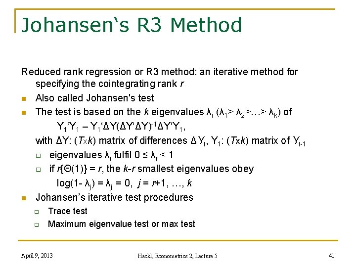
Johansen‘s R 3 Method Reduced rank regression or R 3 method: an iterative method for specifying the cointegrating rank r n Also called Johansen's test n The test is based on the k eigenvalues λi (λ 1> λ 2>…> λk) of Y 1‘Y 1 – Y 1‘ΔY(ΔY‘ΔY)-1ΔY‘Y 1, with ΔY: (Txk) matrix of differences ΔYt, Y 1: (Txk) matrix of Yt-1 q eigenvalues λi fulfil 0 ≤ λi < 1 q if r{Θ(1)} = r, the k-r smallest eigenvalues obey log(1 - λj) = λj = 0, j = r+1, …, k n Johansen’s iterative test procedures q q Trace test Maximum eigenvalue test or max test April 9, 2013 Hackl, Econometrics 2, Lecture 5 41

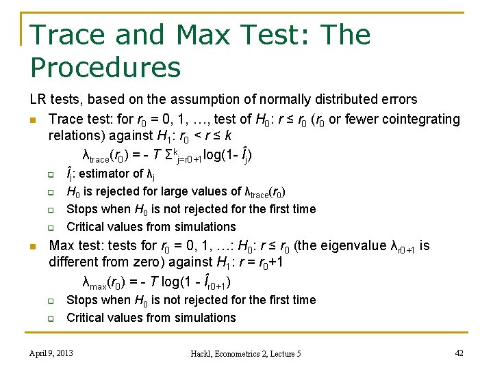
Trace and Max Test: The Procedures LR tests, based on the assumption of normally distributed errors n Trace test: for r 0 = 0, 1, …, test of H 0: r ≤ r 0 (r 0 or fewer cointegrating relations) against H 1: r 0 < r ≤ k λtrace(r 0) = - T Σkj=r 0+1 log(1 - Îj) q q n Îj: estimator of λj H 0 is rejected for large values of λtrace(r 0) Stops when H 0 is not rejected for the first time Critical values from simulations Max test: tests for r 0 = 0, 1, …: H 0: r ≤ r 0 (the eigenvalue λr 0+1 is different from zero) against H 1: r = r 0+1 λmax(r 0) = - T log(1 - Îr 0+1) q q Stops when H 0 is not rejected for the first time Critical values from simulations April 9, 2013 Hackl, Econometrics 2, Lecture 5 42

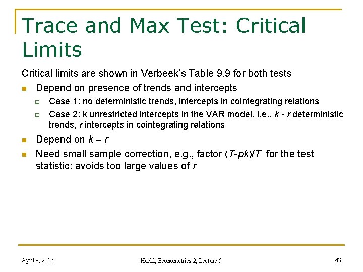
Trace and Max Test: Critical Limits Critical limits are shown in Verbeek’s Table 9. 9 for both tests n Depend on presence of trends and intercepts q q n n Case 1: no deterministic trends, intercepts in cointegrating relations Case 2: k unrestricted intercepts in the VAR model, i. e. , k - r deterministic trends, r intercepts in cointegrating relations Depend on k – r Need small sample correction, e. g. , factor (T-pk)/T for the test statistic: avoids too large values of r April 9, 2013 Hackl, Econometrics 2, Lecture 5 43

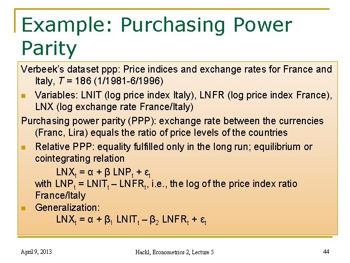
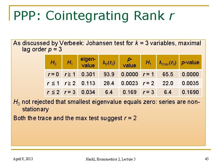
Example: Purchasing Power Parity Verbeek’s dataset ppp: Price indices and exchange rates for France and Italy, T = 186 (1/1981 -6/1996) n Variables: LNIT (log price index Italy), LNFR (log price index France), LNX (log exchange rate France/Italy) Purchasing power parity (PPP): exchange rate between the currencies (Franc, Lira) equals the ratio of price levels of the countries n Relative PPP: equality fulfilled only in the long run; equilibrium or cointegrating relation LNXt = α + β LNPt + εt with LNPt = LNITt – LNFRt, i. e. , the log of the price index ratio France/Italy n Generalization: LNXt = α + β 1 LNITt – β 2 LNFRt + εt April 9, 2013 Hackl, Econometrics 2, Lecture 5 44

PPP: Cointegrating Rank r As discussed by Verbeek: Johansen test for k = 3 variables, maximal lag order p = 3 eigenvalue λtr(r 0) r=0 r≥ 1 0. 301 93. 9 0. 0000 r = 1 65. 5 0. 0000 r ≤ 1 r≥ 2 0. 113 28. 4 0. 0023 r = 2 22. 0 0. 0035 r ≤ 2 r=3 0. 034 6. 4 0. 1690 H 1 pvalue H 1 r=3 λmax(r 0) p-value H 0 not rejected that smallest eigenvalue equals zero: series are nonstationary Both the trace and the max test suggest r = 2 April 9, 2013 Hackl, Econometrics 2, Lecture 5 45

Contents n n n Systems of Equations VAR Models Simultaneous Equations and VAR Models and Cointegration VEC Model: Cointegration Tests VEC Model: Specification and Estimation April 9, 2013 Hackl, Econometrics 2, Lecture 5 46

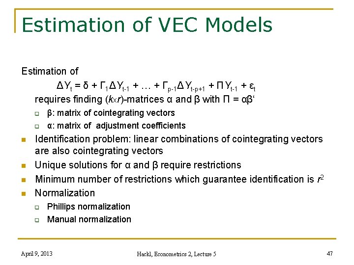
Estimation of VEC Models Estimation of ΔYt = δ + Γ 1ΔYt-1 + … + Γp-1ΔYt-p+1 + ΠYt-1 + εt requires finding (kxr)-matrices α and β with Π = αβ‘ q q n n β: matrix of cointegrating vectors α: matrix of adjustment coefficients Identification problem: linear combinations of cointegrating vectors are also cointegrating vectors Unique solutions for α and β require restrictions Minimum number of restrictions which guarantee identification is r 2 Normalization q q Phillips normalization Manual normalization April 9, 2013 Hackl, Econometrics 2, Lecture 5 47

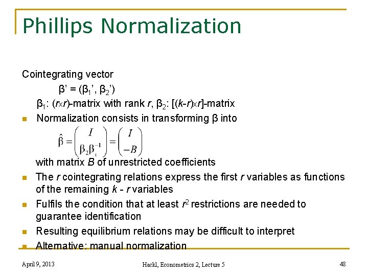
Phillips Normalization Cointegrating vector β’ = (β 1’, β 2’) β 1: (rxr)-matrix with rank r, β 2: [(k-r)xr]-matrix n Normalization consists in transforming β into n n with matrix B of unrestricted coefficients The r cointegrating relations express the first r variables as functions of the remaining k - r variables Fulfils the condition that at least r 2 restrictions are needed to guarantee identification Resulting equilibrium relations may be difficult to interpret Alternative: manual normalization April 9, 2013 Hackl, Econometrics 2, Lecture 5 48

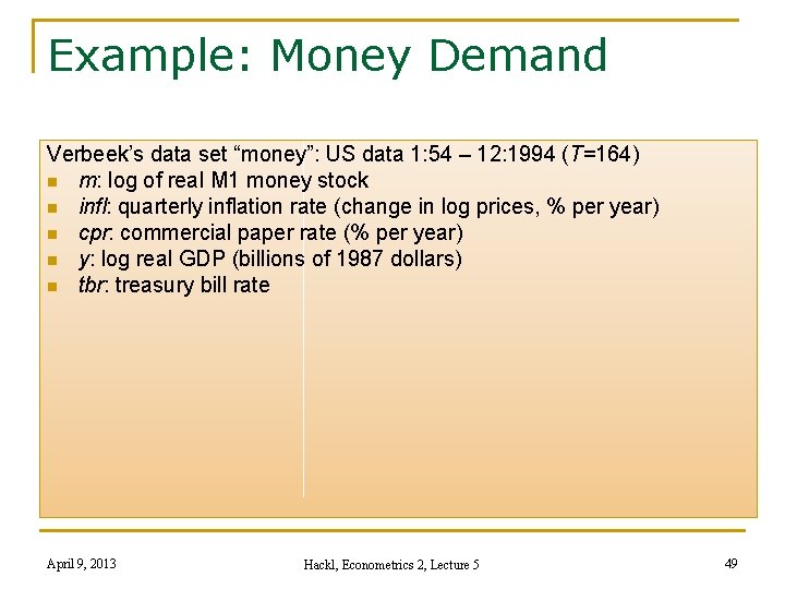
Example: Money Demand Verbeek’s data set “money”: US data 1: 54 – 12: 1994 (T=164) n m: log of real M 1 money stock n infl: quarterly inflation rate (change in log prices, % per year) n cpr: commercial paper rate (% per year) n y: log real GDP (billions of 1987 dollars) n tbr: treasury bill rate April 9, 2013 Hackl, Econometrics 2, Lecture 5 49

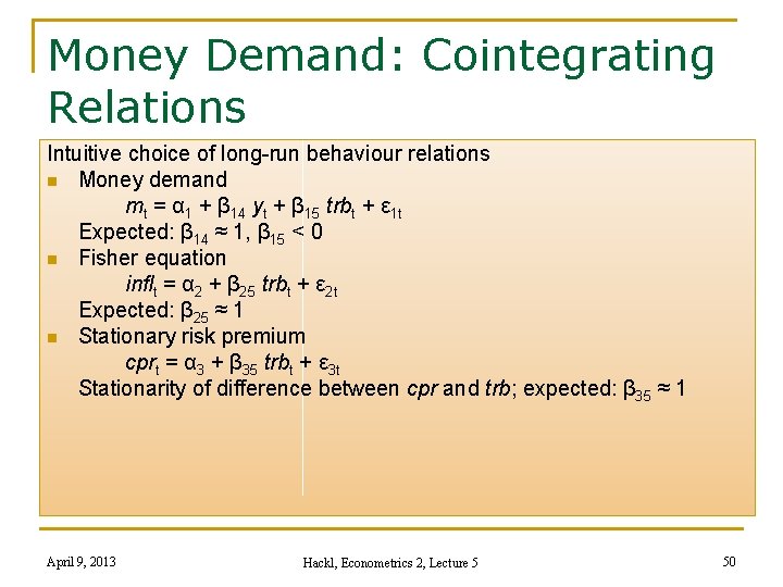
Money Demand: Cointegrating Relations Intuitive choice of long-run behaviour relations n Money demand mt = α 1 + β 14 yt + β 15 trbt + ε 1 t Expected: β 14 ≈ 1, β 15 < 0 n Fisher equation inflt = α 2 + β 25 trbt + ε 2 t Expected: β 25 ≈ 1 n Stationary risk premium cprt = α 3 + β 35 trbt + ε 3 t Stationarity of difference between cpr and trb; expected: β 35 ≈ 1 April 9, 2013 Hackl, Econometrics 2, Lecture 5 50

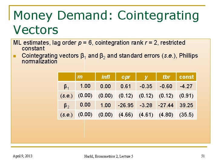
Money Demand: Cointegrating Vectors ML estimates, lag order p = 6, cointegration rank r = 2, restricted constant n Cointegrating vectors β 1 and β 2 and standard errors (s. e. ), Phillips normalization m April 9, 2013 infl cpr y tbr const β 1 1. 00 0. 61 -0. 35 -0. 60 -4. 27 (s. e. ) (0. 00) (0. 12) (0. 91) β 2 0. 00 1. 00 -26. 95 -3. 28 -27. 44 39. 25 (s. e. ) (0. 00) (4. 66) (4. 61) (4. 80) (35. 5) Hackl, Econometrics 2, Lecture 5 51

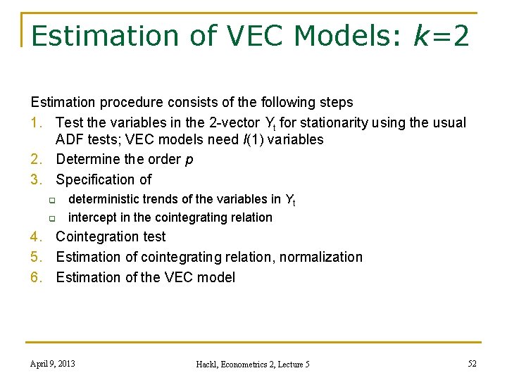
Estimation of VEC Models: k=2 Estimation procedure consists of the following steps 1. Test the variables in the 2 -vector Yt for stationarity using the usual ADF tests; VEC models need I(1) variables 2. Determine the order p 3. Specification of q q deterministic trends of the variables in Yt intercept in the cointegrating relation 4. Cointegration test 5. Estimation of cointegrating relation, normalization 6. Estimation of the VEC model April 9, 2013 Hackl, Econometrics 2, Lecture 5 52

Example: Income and Consumption Model: Yt = δ 1 + θ 11 Yt-1 + θ 12 Ct-1 + ε 1 t Ct = δ 2 + θ 21 Ct-1 + θ 22 Yt-1 + ε 2 t With Z = (Y, C)‘, 2 -vectors δ and ε, and (2 x 2)-matrix Θ, the VAR(1) model is Zt = δ + ΘZt-1 + εt Represents each component of Z as a linear combination of lagged variables April 9, 2013 Hackl, Econometrics 2, Lecture 5 53

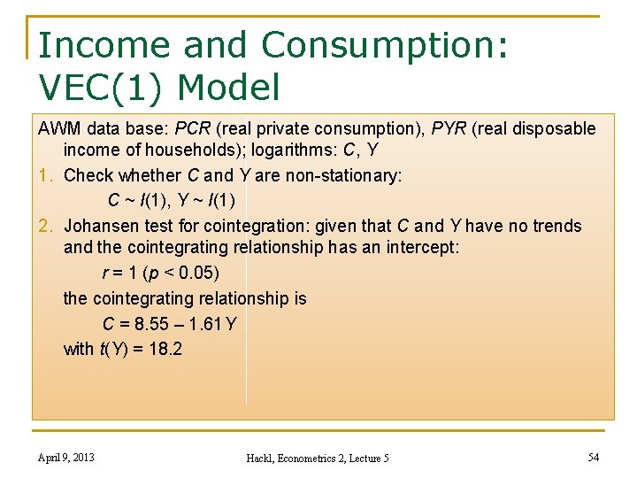
Income and Consumption: VEC(1) Model AWM data base: PCR (real private consumption), PYR (real disposable income of households); logarithms: C, Y 1. Check whether C and Y are non-stationary: C ~ I(1), Y ~ I(1) 2. Johansen test for cointegration: given that C and Y have no trends and the cointegrating relationship has an intercept: r = 1 (p < 0. 05) the cointegrating relationship is C = 8. 55 – 1. 61 Y with t(Y) = 18. 2 April 9, 2013 Hackl, Econometrics 2, Lecture 5 54

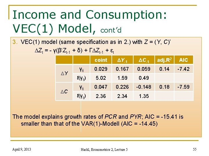
Income and Consumption: VEC(1) Model, cont’d 3. VEC(1) model (same specification as in 2. ) with Z = (Y, C)’ DZt = - γ(β‘Zt-1 + δ) + ΓDZt-1 + εt DY DC coint DY-1 DC-1 adj. R 2 AIC γij 0. 029 0. 167 0. 059 0. 14 -7. 42 t(γij) 5. 02 1. 59 0. 49 γij 0. 047 0. 226 -0. 148 0. 18 -7. 59 t(γij) 2. 36 2. 34 1. 35 The model explains growth rates of PCR and PYR; AIC = -15. 41 is smaller than that of the VAR(1)-Modell (AIC = -14. 45) April 9, 2013 Hackl, Econometrics 2, Lecture 5 55

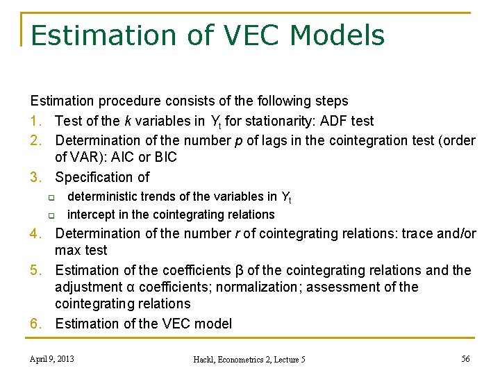
Estimation of VEC Models Estimation procedure consists of the following steps 1. Test of the k variables in Yt for stationarity: ADF test 2. Determination of the number p of lags in the cointegration test (order of VAR): AIC or BIC 3. Specification of q q deterministic trends of the variables in Yt intercept in the cointegrating relations 4. Determination of the number r of cointegrating relations: trace and/or max test 5. Estimation of the coefficients β of the cointegrating relations and the adjustment α coefficients; normalization; assessment of the cointegrating relations 6. Estimation of the VEC model April 9, 2013 Hackl, Econometrics 2, Lecture 5 56

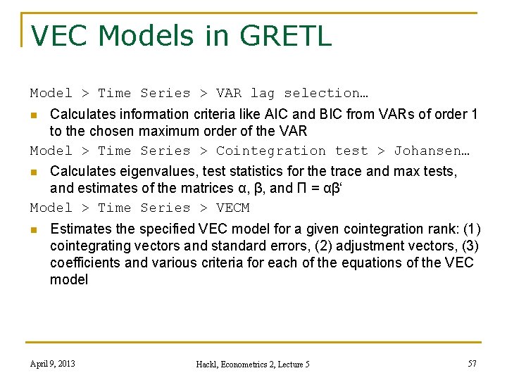
VEC Models in GRETL Model > Time Series > VAR lag selection… Calculates information criteria like AIC and BIC from VARs of order 1 to the chosen maximum order of the VAR Model > Time Series > Cointegration test > Johansen… n Calculates eigenvalues, test statistics for the trace and max tests, and estimates of the matrices α, β, and Π = αβ‘ Model > Time Series > VECM n n Estimates the specified VEC model for a given cointegration rank: (1) cointegrating vectors and standard errors, (2) adjustment vectors, (3) coefficients and various criteria for each of the equations of the VEC model April 9, 2013 Hackl, Econometrics 2, Lecture 5 57

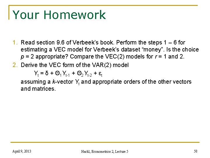
Your Homework 1. Read section 9. 6 of Verbeek’s book. Perform the steps 1 – 6 for estimating a VEC model for Verbeek’s dataset “money”. Is the choice p = 2 appropriate? Compare the VEC(2) models for r = 1 and 2. 2. Derive the VEC form of the VAR(2) model Yt = δ + Θ 1 Yt-1 + Θ 2 Yt-2 + εt assuming a k-vector Yt and appropriate orders of the other vectors and matrices. April 9, 2013 Hackl, Econometrics 2, Lecture 5 58