Econometrics 2 Lecture 3 Univariate Time Series Models

Econometrics 2 - Lecture 3 Univariate Time Series Models

Contents n n n n Time Series Stochastic Processes Stationary Processes The ARMA Process Deterministic and Stochastic Trends Models with Trend Unit Root Tests Estimation of ARMA Models March 23, 2018 Hackl, Econometrics 2, Lecture 3 2

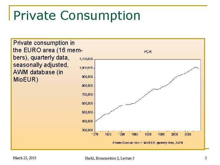
Private Consumption Private consumption in the EURO area (16 members), quarterly data, seasonally adjusted, AWM database (in Mio. EUR) March 23, 2018 Hackl, Econometrics 2, Lecture 3 3

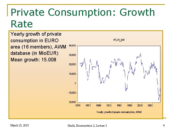
Private Consumption: Growth Rate Yearly growth of private consumption in EURO area (16 members), AWM database (in Mio. EUR) Mean growth: 15. 008 March 23, 2018 Hackl, Econometrics 2, Lecture 3 4

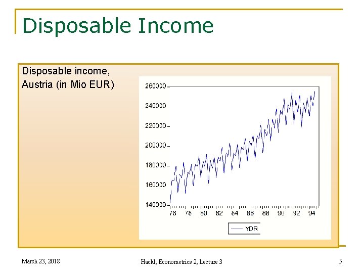
Disposable Income Disposable income, Austria (in Mio EUR) March 23, 2018 Hackl, Econometrics 2, Lecture 3 5

Time Series Time-ordered sequence of observations of a random variable Examples: n Annual values of private consumption n Yearly changes in expenditures on private consumption n Quarterly values of personal disposable income n Monthly values of imports Notation: n Random variable Y n Sequence of observations Y 1, Y 2, . . . , YT n Deviations from the mean: yt = Yt – E{Yt} = Yt – μ March 23, 2018 Hackl, Econometrics 2, Lecture 3 6

Components of a Time Series Components or characteristics of a time series are n Trend n Seasonality n Irregular fluctuations Time series model: represents the characteristics as well as possible interactions Purpose of modelling n Description of the time series n Forecasting the future Example: Quarterly observations of the disposable income Yt = βt + Σiγi. Dit + εt with Dit = 1 if t corresponds to i-th quarter, Dit = 0 otherwise March 23, 2018 Hackl, Econometrics 2, Lecture 3 7

Contents n n n n Time Series Stochastic Processes Stationary Processes The ARMA Process Deterministic and Stochastic Trends Models with Trend Unit Root Tests Estimation of ARMA Models March 23, 2018 Hackl, Econometrics 2, Lecture 3 8

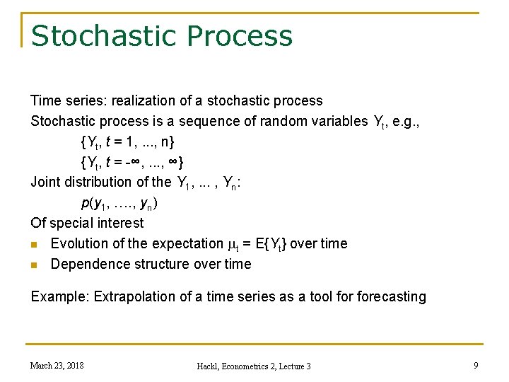
Stochastic Process Time series: realization of a stochastic process Stochastic process is a sequence of random variables Yt, e. g. , {Yt, t = 1, . . . , n} {Yt, t = -∞, . . . , ∞} Joint distribution of the Y 1, . . . , Yn: p(y 1, …. , yn) Of special interest n Evolution of the expectation mt = E{Yt} over time n Dependence structure over time Example: Extrapolation of a time series as a tool forecasting March 23, 2018 Hackl, Econometrics 2, Lecture 3 9

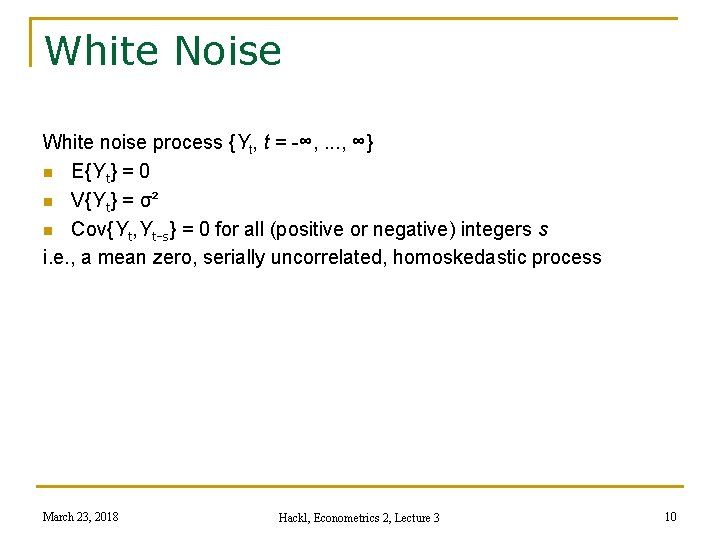
White Noise White noise process {Yt, t = -∞, . . . , ∞} n E{Yt} = 0 n V{Yt} = σ² n Cov{Yt, Yt-s} = 0 for all (positive or negative) integers s i. e. , a mean zero, serially uncorrelated, homoskedastic process March 23, 2018 Hackl, Econometrics 2, Lecture 3 10

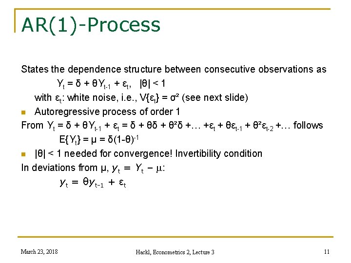
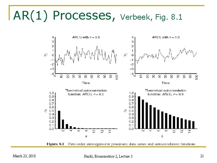
AR(1)-Process States the dependence structure between consecutive observations as Yt = δ + θYt-1 + εt, |θ| < 1 with εt: white noise, i. e. , V{εt} = σ² (see next slide) n Autoregressive process of order 1 From Yt = δ + θYt-1 + εt = δ + θ²δ +… +εt + θεt-1 + θ²εt-2 +… follows E{Yt} = μ = δ(1 -θ)-1 n |θ| < 1 needed for convergence! Invertibility condition In deviations from μ, yt = Yt – m: yt = θyt-1 + εt March 23, 2018 Hackl, Econometrics 2, Lecture 3 11

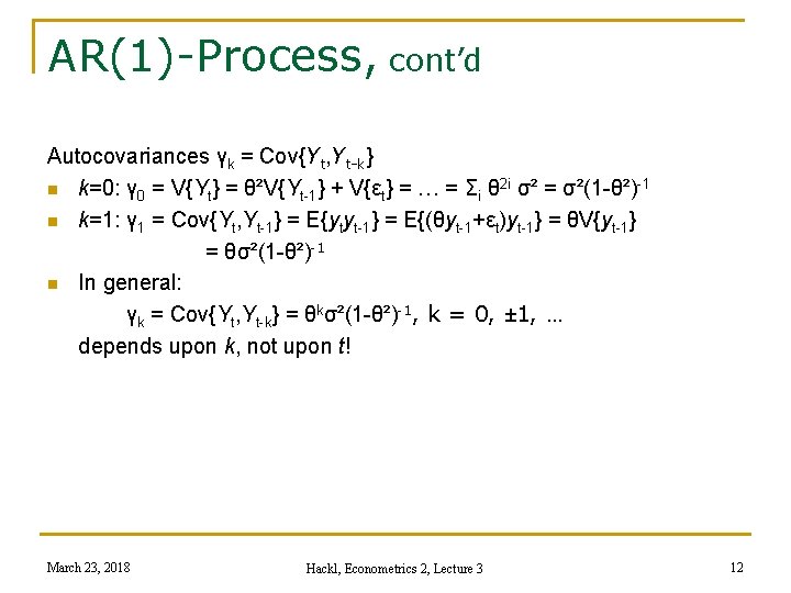
AR(1)-Process, cont’d Autocovariances γk = Cov{Yt, Yt-k} n k=0: γ 0 = V{Yt} = θ²V{Yt-1} + V{εt} = … = Σi θ 2 i σ² = σ²(1 -θ²)-1 n k=1: γ 1 = Cov{Yt, Yt-1} = E{ytyt-1} = E{(θyt-1+εt)yt-1} = θV{yt-1} = θσ²(1 -θ²)-1 n In general: γk = Cov{Yt, Yt-k} = θkσ²(1 -θ²)-1, k = 0, ± 1, … depends upon k, not upon t! March 23, 2018 Hackl, Econometrics 2, Lecture 3 12

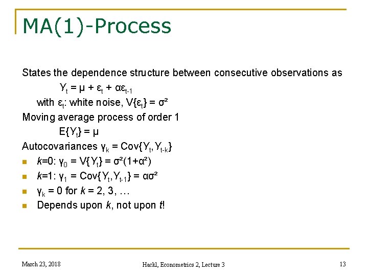
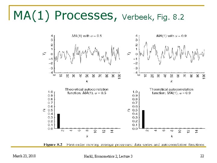
MA(1)-Process States the dependence structure between consecutive observations as Yt = μ + εt + αεt-1 with εt: white noise, V{εt} = σ² Moving average process of order 1 E{Yt} = μ Autocovariances γk = Cov{Yt, Yt-k} n k=0: γ 0 = V{Yt} = σ²(1+α²) n k=1: γ 1 = Cov{Yt, Yt-1} = ασ² n γk = 0 for k = 2, 3, … n Depends upon k, not upon t! March 23, 2018 Hackl, Econometrics 2, Lecture 3 13

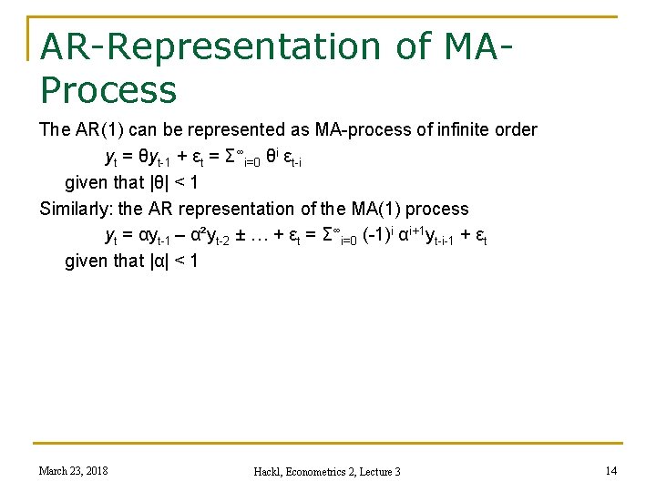
AR-Representation of MAProcess The AR(1) can be represented as MA-process of infinite order yt = θyt-1 + εt = Σ∞i=0 θi εt-i given that |θ| < 1 Similarly: the AR representation of the MA(1) process yt = αyt-1 – α²yt-2 ± … + εt = Σ∞i=0 (-1)i αi+1 yt-i-1 + εt given that |α| < 1 March 23, 2018 Hackl, Econometrics 2, Lecture 3 14

Contents n n n n Time Series Stochastic Processes Stationary Processes The ARMA Process Deterministic and Stochastic Trends Models with Trend Unit Root Tests Estimation of ARMA Models March 23, 2018 Hackl, Econometrics 2, Lecture 3 15

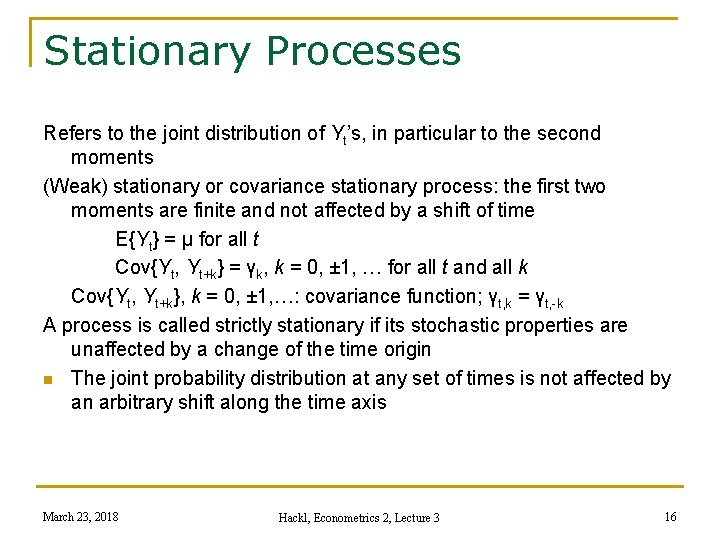
Stationary Processes Refers to the joint distribution of Yt’s, in particular to the second moments (Weak) stationary or covariance stationary process: the first two moments are finite and not affected by a shift of time E{Yt} = μ for all t Cov{Yt, Yt+k} = γk, k = 0, ± 1, … for all t and all k Cov{Yt, Yt+k}, k = 0, ± 1, …: covariance function; γt, k = γt, -k A process is called strictly stationary if its stochastic properties are unaffected by a change of the time origin n The joint probability distribution at any set of times is not affected by an arbitrary shift along the time axis March 23, 2018 Hackl, Econometrics 2, Lecture 3 16

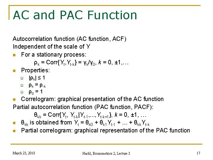
AC and PAC Function Autocorrelation function (AC function, ACF) Independent of the scale of Y n For a stationary process: ρk = Corr{Yt, Yt-k} = γk/γ 0, k = 0, ± 1, … n Properties: q q q |ρk| ≤ 1 ρk = ρ-k ρ0 = 1 Correlogram: graphical presentation of the AC function Partial autocorrelation function (PAC function, PACF): θkk = Corr{Yt, Yt-k|Yt-1, . . . , Yt-k+1}, k = 0, ± 1, … n θkk is obtained from Yt = θk 0 + θk 1 Yt-1 +. . . + θkk. Yt-k n Partial correlogram: graphical representation of the PAC function n March 23, 2018 Hackl, Econometrics 2, Lecture 3 17

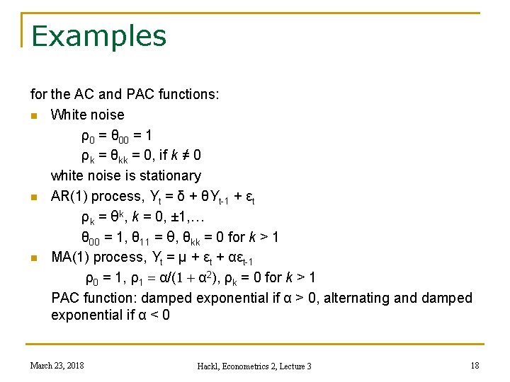
Examples for the AC and PAC functions: n White noise ρ0 = θ 00 = 1 ρk = θkk = 0, if k ≠ 0 white noise is stationary n AR(1) process, Yt = δ + θYt-1 + εt ρk = θk, k = 0, ± 1, … θ 00 = 1, θ 11 = θ, θkk = 0 for k > 1 n MA(1) process, Yt = μ + εt + αεt-1 ρ0 = 1, ρ1 = α/(1 + α 2), ρk = 0 for k > 1 PAC function: damped exponential if α > 0, alternating and damped exponential if α < 0 March 23, 2018 Hackl, Econometrics 2, Lecture 3 18

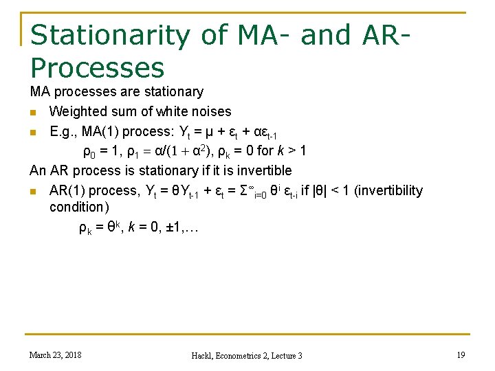
Stationarity of MA- and ARProcesses MA processes are stationary n Weighted sum of white noises n E. g. , MA(1) process: Yt = μ + εt + αεt-1 ρ0 = 1, ρ1 = α/(1 + α 2), ρk = 0 for k > 1 An AR process is stationary if it is invertible n AR(1) process, Yt = θYt-1 + εt = Σ∞i=0 θi εt-i if |θ| < 1 (invertibility condition) ρk = θk, k = 0, ± 1, … March 23, 2018 Hackl, Econometrics 2, Lecture 3 19

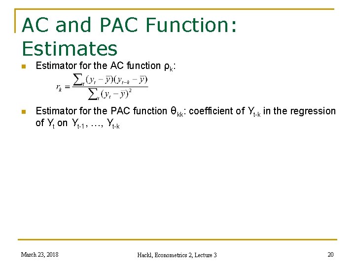
AC and PAC Function: Estimates n Estimator for the AC function ρk: n Estimator for the PAC function θkk: coefficient of Yt-k in the regression of Yt on Yt-1, …, Yt-k March 23, 2018 Hackl, Econometrics 2, Lecture 3 20

AR(1) Processes, March 23, 2018 Verbeek, Fig. 8. 1 Hackl, Econometrics 2, Lecture 3 21

MA(1) Processes, March 23, 2018 Verbeek, Fig. 8. 2 Hackl, Econometrics 2, Lecture 3 22

Contents n n n n Time Series Stochastic Processes Stationary Processes The ARMA Process Deterministic and Stochastic Trends Models with Trend Unit Root Tests Estimation of ARMA Models March 23, 2018 Hackl, Econometrics 2, Lecture 3 23

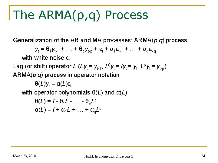
The ARMA(p, q) Process Generalization of the AR and MA processes: ARMA(p, q) process yt = θ 1 yt-1 + … + θpyt-p + εt + α 1εt-1 + … + αqεt-q with white noise εt Lag (or shift) operator L (Lyt = yt-1, L 0 yt = Iyt = yt, Lpyt = yt-p) ARMA(p, q) process in operator notation θ(L)yt = α(L)εt with operator polynomials θ(L) and α(L) θ(L) = I - θ 1 L - … - θp. Lp α(L) = I + α 1 L + … + αq. Lq March 23, 2018 Hackl, Econometrics 2, Lecture 3 24

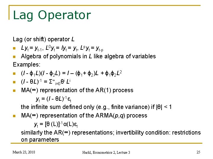
Lag Operator Lag (or shift) operator L n Lyt = yt-1, L 0 yt = Iyt = yt, Lpyt = yt-p n Algebra of polynomials in L like algebra of variables Examples: n (I - ϕ 1 L)(I - ϕ 2 L) = I – (ϕ 1+ ϕ 2)L + ϕ 1ϕ 2 L 2 n (I - θL)-1 = Σ∞i=0θi Li n MA(∞) representation of the AR(1) process yt = (I - θL)-1εt the infinite sum defined only (e. g. , finite variance) if |θ| < 1 n MA(∞) representation of the ARMA(p, q) process yt = [θ (L)]-1α(L)εt similarly the AR(∞) representations; invertibility condition: restrictions on parameters March 23, 2018 Hackl, Econometrics 2, Lecture 3 25

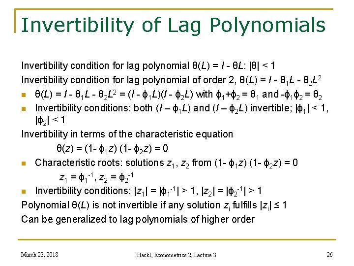
Invertibility of Lag Polynomials Invertibility condition for lag polynomial θ(L) = I - θL: |θ| < 1 Invertibility condition for lag polynomial of order 2, θ(L) = I - θ 1 L - θ 2 L 2 n θ(L) = I - θ 1 L - θ 2 L 2 = (I - ϕ 1 L)(I - ϕ 2 L) with ϕ 1+ϕ 2 = θ 1 and -ϕ 1ϕ 2 = θ 2 n Invertibility conditions: both (I – ϕ 1 L) and (I – ϕ 2 L) invertible; |ϕ 1| < 1, |ϕ 2| < 1 Invertibility in terms of the characteristic equation θ(z) = (1 - ϕ 1 z) (1 - ϕ 2 z) = 0 n Characteristic roots: solutions z 1, z 2 from (1 - ϕ 1 z) (1 - ϕ 2 z) = 0 z 1 = ϕ 1 -1, z 2 = ϕ 2 -1 n Invertibility conditions: |z 1| = |ϕ 1 -1| > 1, |z 2| = |ϕ 2 -1| > 1 Polynomial θ(L) is not invertible if any solution zi fulfills |zi| ≤ 1 Can be generalized to lag polynomials of higher order March 23, 2018 Hackl, Econometrics 2, Lecture 3 26

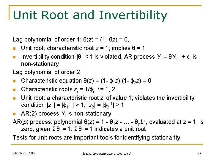
Unit Root and Invertibility Lag polynomial of order 1: θ(z) = (1 - θz) = 0, n Unit root: characteristic root z = 1; implies θ = 1 n Invertibility condition |θ| < 1 is violated, AR process Yt = θYt-1 + εt is non-stationary Lag polynomial of order 2 n Characteristic equation θ(z) = (1 - ϕ 1 z) (1 - ϕ 2 z) = 0 n Characteristic roots zi = 1/ϕi, i = 1, 2 n Unit root: a characteristic root zi of value 1; violates the invertibility condition |z 1| = |ϕ 1 -1| > 1, |z 2| = |ϕ 2 -1| > 1 n AR(2) process Yt is non-stationary AR(p) process: polynomial θ(z) = 1 - θ 1 z - … - θp. Lp, evaluated at z = 1, is zero, given Σiθi = 1: Σiθi = 1 indicates a unit root Tests for unit roots are important tools for identifying stationarity March 23, 2018 Hackl, Econometrics 2, Lecture 3 27

Contents n n n n Time Series Stochastic Processes Stationary Processes The ARMA Process Deterministic and Stochastic Trends Models with Trend Unit Root Tests Estimation of ARMA Models March 23, 2018 Hackl, Econometrics 2, Lecture 3 28

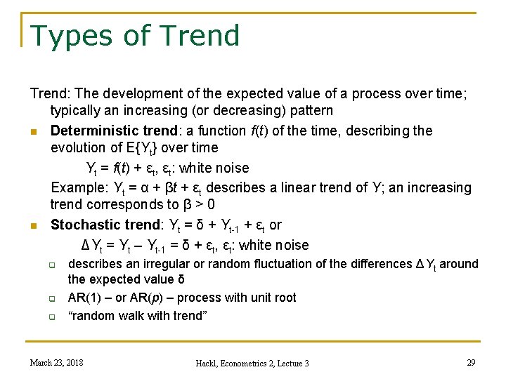
Types of Trend: The development of the expected value of a process over time; typically an increasing (or decreasing) pattern n Deterministic trend: a function f(t) of the time, describing the evolution of E{Yt} over time Yt = f(t) + εt, εt: white noise Example: Yt = α + βt + εt describes a linear trend of Y; an increasing trend corresponds to β > 0 n Stochastic trend: Yt = δ + Yt-1 + εt or ΔYt = Yt – Yt-1 = δ + εt, εt: white noise q q q describes an irregular or random fluctuation of the differences ΔYt around the expected value δ AR(1) – or AR(p) – process with unit root “random walk with trend” March 23, 2018 Hackl, Econometrics 2, Lecture 3 29

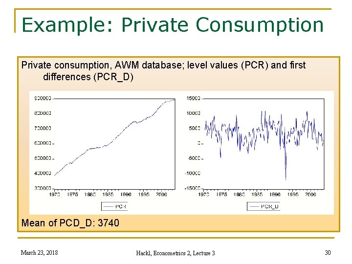
Example: Private Consumption Private consumption, AWM database; level values (PCR) and first differences (PCR_D) Mean of PCD_D: 3740 March 23, 2018 Hackl, Econometrics 2, Lecture 3 30

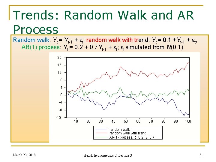
Trends: Random Walk and AR Process Random walk: Yt = Yt-1 + εt; random walk with trend: Yt = 0. 1 +Yt-1 + εt; AR(1) process: Yt = 0. 2 + 0. 7 Yt-1 + εt; εt simulated from N(0, 1) 20 16 12 8 4 0 -4 -8 -12 10 20 30 40 50 60 70 80 90 100 random walk with trend AR(1) process, δ=0. 2, θ=0. 7 March 23, 2018 Hackl, Econometrics 2, Lecture 3 31

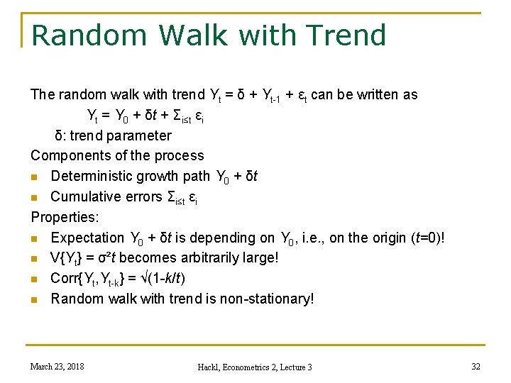
Random Walk with Trend The random walk with trend Yt = δ + Yt-1 + εt can be written as Yt = Y 0 + δt + Σi≤t εi δ: trend parameter Components of the process n Deterministic growth path Y 0 + δt n Cumulative errors Σi≤t εi Properties: n Expectation Y 0 + δt is depending on Y 0, i. e. , on the origin (t=0)! n V{Yt} = σ²t becomes arbitrarily large! n Corr{Yt, Yt-k} = √(1 -k/t) n Random walk with trend is non-stationary! March 23, 2018 Hackl, Econometrics 2, Lecture 3 32

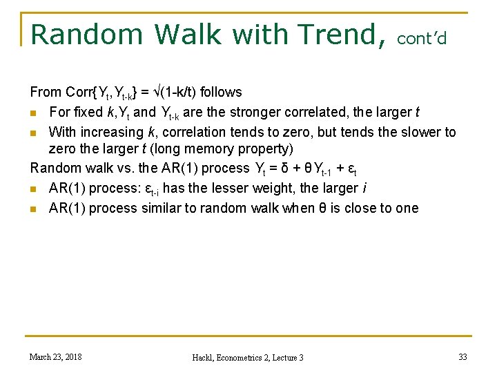
Random Walk with Trend, cont’d From Corr{Yt, Yt-k} = √(1 -k/t) follows n For fixed k, Yt and Yt-k are the stronger correlated, the larger t n With increasing k, correlation tends to zero, but tends the slower to zero the larger t (long memory property) Random walk vs. the AR(1) process Yt = δ + θYt-1 + εt n AR(1) process: εt-i has the lesser weight, the larger i n AR(1) process similar to random walk when θ is close to one March 23, 2018 Hackl, Econometrics 2, Lecture 3 33

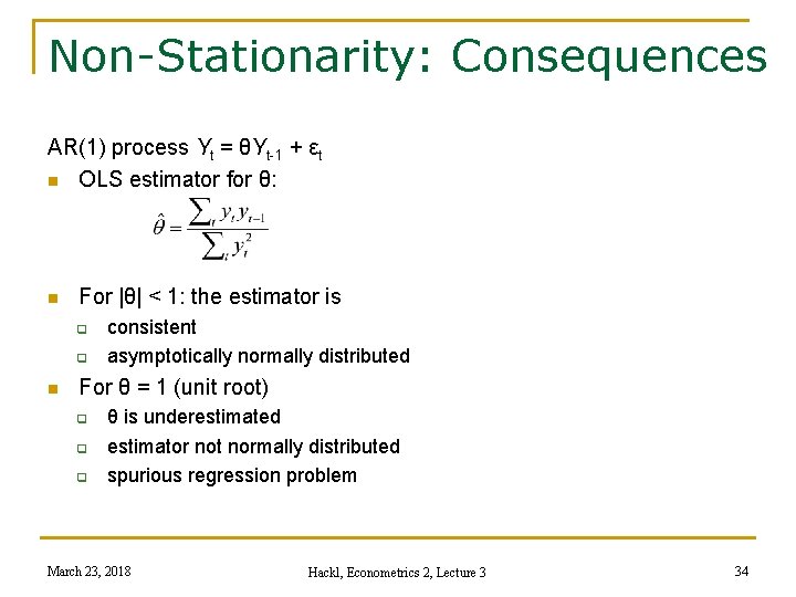
Non-Stationarity: Consequences AR(1) process Yt = θYt-1 + εt n OLS estimator for θ: n For |θ| < 1: the estimator is q q n consistent asymptotically normally distributed For θ = 1 (unit root) q q q θ is underestimated estimator not normally distributed spurious regression problem March 23, 2018 Hackl, Econometrics 2, Lecture 3 34

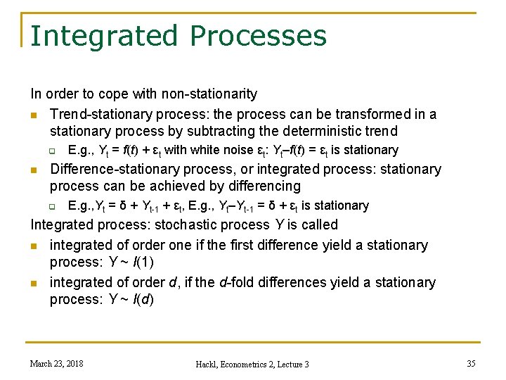
Integrated Processes In order to cope with non-stationarity n Trend-stationary process: the process can be transformed in a stationary process by subtracting the deterministic trend q n E. g. , Yt = f(t) + εt with white noise εt: Yt–f(t) = εt is stationary Difference-stationary process, or integrated process: stationary process can be achieved by differencing q E. g. , Yt = δ + Yt-1 + εt, E. g. , Yt–Yt-1 = δ + εt is stationary Integrated process: stochastic process Y is called n integrated of order one if the first difference yield a stationary process: Y ~ I(1) n integrated of order d, if the d-fold differences yield a stationary process: Y ~ I(d) March 23, 2018 Hackl, Econometrics 2, Lecture 3 35

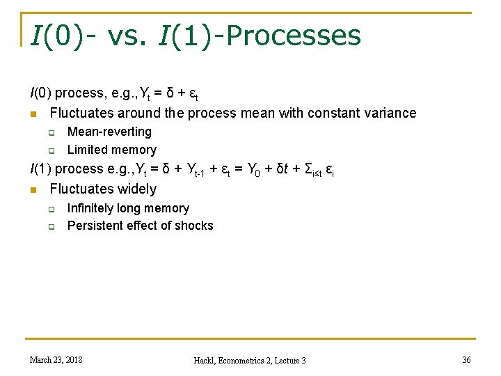
I(0)- vs. I(1)-Processes I(0) process, e. g. , Yt = δ + εt n Fluctuates around the process mean with constant variance q q Mean-reverting Limited memory I(1) process e. g. , Yt = δ + Yt-1 + εt = Y 0 + δt + Σi≤t εi n Fluctuates widely q q Infinitely long memory Persistent effect of shocks March 23, 2018 Hackl, Econometrics 2, Lecture 3 36

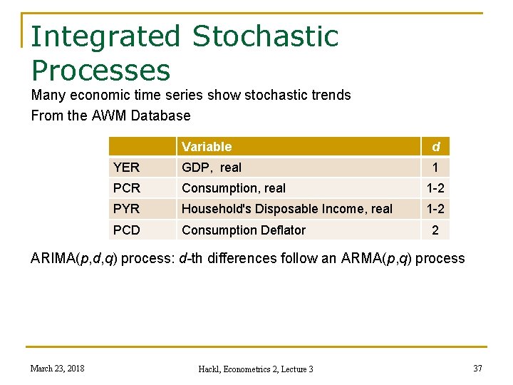
Integrated Stochastic Processes Many economic time series show stochastic trends From the AWM Database Variable d YER GDP, real 1 PCR Consumption, real 1 -2 PYR Household's Disposable Income, real 1 -2 PCD Consumption Deflator 2 ARIMA(p, d, q) process: d-th differences follow an ARMA(p, q) process March 23, 2018 Hackl, Econometrics 2, Lecture 3 37

Contents n n n n Time Series Stochastic Processes Stationary Processes The ARMA Process Deterministic and Stochastic Trends Models with Trend Unit Root Tests Estimation of ARMA Models March 23, 2018 Hackl, Econometrics 2, Lecture 3 38

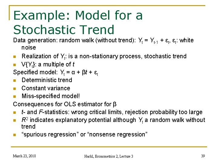
Example: Model for a Stochastic Trend Data generation: random walk (without trend): Yt = Yt-1 + εt, εt: white noise n Realization of Yt: is a non-stationary process, stochastic trend n V{Yt}: a multiple of t Specified model: Yt = α + βt + εt n Deterministic trend n Constant variance n Miss-specified model! Consequences for OLS estimator for β n t- and F-statistics: wrong critical limits, rejection probability too large n R 2 indicates explanatory potential although Yt a random walk without trend n “spurious regression” or “nonsense regression” March 23, 2018 Hackl, Econometrics 2, Lecture 3 39

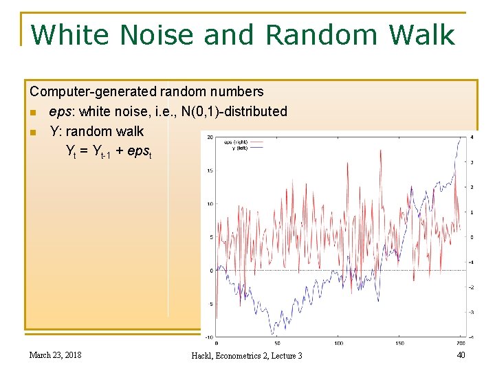
White Noise and Random Walk Computer-generated random numbers n eps: white noise, i. e. , N(0, 1)-distributed n Y: random walk Yt = Yt-1 + epst March 23, 2018 Hackl, Econometrics 2, Lecture 3 40

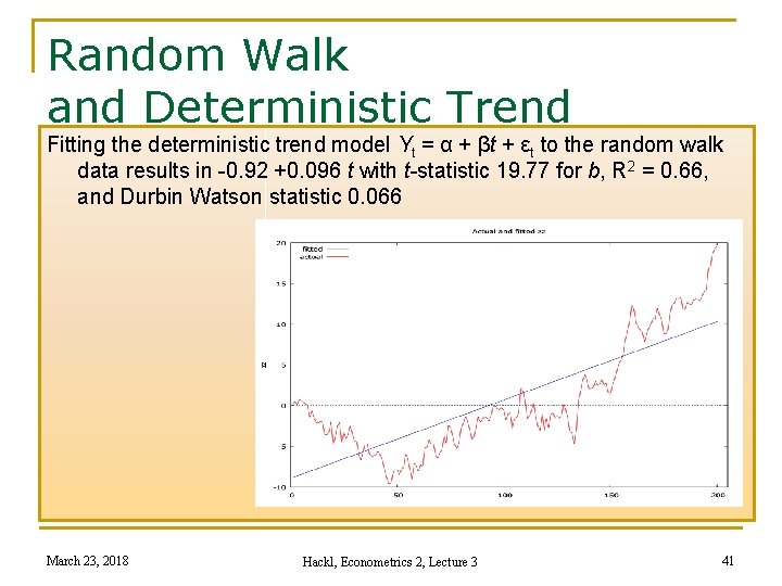
Random Walk and Deterministic Trend Fitting the deterministic trend model Yt = α + βt + εt to the random walk data results in -0. 92 +0. 096 t with t-statistic 19. 77 for b, R 2 = 0. 66, and Durbin Watson statistic 0. 066 March 23, 2018 Hackl, Econometrics 2, Lecture 3 41

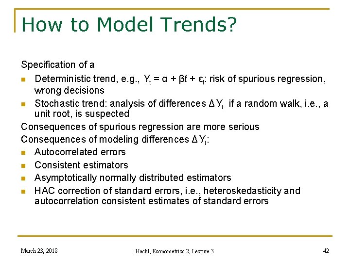
How to Model Trends? Specification of a n Deterministic trend, e. g. , Yt = α + βt + εt: risk of spurious regression, wrong decisions n Stochastic trend: analysis of differences ΔYt if a random walk, i. e. , a unit root, is suspected Consequences of spurious regression are more serious Consequences of modeling differences ΔYt: n Autocorrelated errors n Consistent estimators n Asymptotically normally distributed estimators n HAC correction of standard errors, i. e. , heteroskedasticity and autocorrelation consistent estimates of standard errors March 23, 2018 Hackl, Econometrics 2, Lecture 3 42

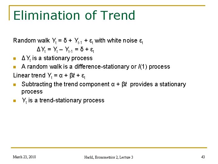
Elimination of Trend Random walk Yt = δ + Yt-1 + εt with white noise εt ΔYt = Yt – Yt-1 = δ + εt n ΔYt is a stationary process n A random walk is a difference-stationary or I(1) process Linear trend Yt = α + βt + εt n Subtracting the trend component α + βt provides a stationary process n Yt is a trend-stationary process March 23, 2018 Hackl, Econometrics 2, Lecture 3 43

Contents n n n n Time Series Stochastic Processes Stationary Processes The ARMA Process Deterministic and Stochastic Trends Models with Trend Unit Root Tests Estimation of ARMA Models March 23, 2018 Hackl, Econometrics 2, Lecture 3 44

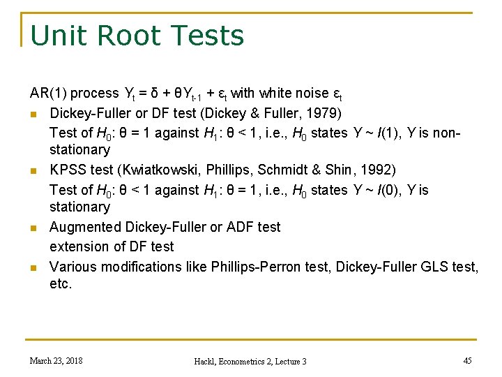
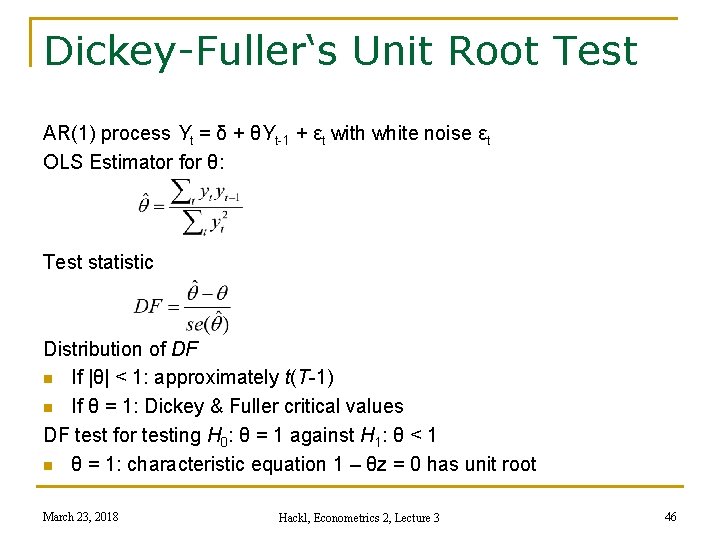
Unit Root Tests AR(1) process Yt = δ + θYt-1 + εt with white noise εt n Dickey-Fuller or DF test (Dickey & Fuller, 1979) Test of H 0: θ = 1 against H 1: θ < 1, i. e. , H 0 states Y ~ I(1), Y is nonstationary n KPSS test (Kwiatkowski, Phillips, Schmidt & Shin, 1992) Test of H 0: θ < 1 against H 1: θ = 1, i. e. , H 0 states Y ~ I(0), Y is stationary n Augmented Dickey-Fuller or ADF test extension of DF test n Various modifications like Phillips-Perron test, Dickey-Fuller GLS test, etc. March 23, 2018 Hackl, Econometrics 2, Lecture 3 45

Dickey-Fuller‘s Unit Root Test AR(1) process Yt = δ + θYt-1 + εt with white noise εt OLS Estimator for θ: Test statistic Distribution of DF n If |θ| < 1: approximately t(T-1) n If θ = 1: Dickey & Fuller critical values DF test for testing H 0: θ = 1 against H 1: θ < 1 n θ = 1: characteristic equation 1 – θz = 0 has unit root March 23, 2018 Hackl, Econometrics 2, Lecture 3 46

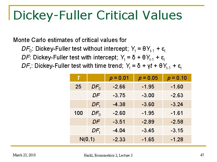
Dickey-Fuller Critical Values Monte Carlo estimates of critical values for DF 0: Dickey-Fuller test without intercept; Yt = θYt-1 + εt DF: Dickey-Fuller test with intercept; Yt = δ + θYt-1 + εt DFτ: Dickey-Fuller test with time trend; Yt = δ + γt + θYt-1 + εt T 25 100 p = 0. 01 p = 0. 05 p = 0. 10 DF 0 -2. 66 -1. 95 -1. 60 DF -3. 75 -3. 00 -2. 63 DFτ -4. 38 -3. 60 -3. 24 DF 0 -2. 60 -1. 95 -1. 61 DF -3. 51 -2. 89 -2. 58 DFτ -4. 04 -3. 45 -3. 15 -2. 33 -1. 65 -1. 28 N(0, 1) March 23, 2018 Hackl, Econometrics 2, Lecture 3 47

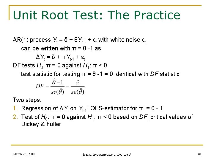
Unit Root Test: The Practice AR(1) process Yt = δ + θYt-1 + εt with white noise εt can be written with π = θ -1 as ΔYt = δ + πYt-1 + εt DF tests H 0: π = 0 against H 1: π < 0 test statistic for testing π = θ -1 = 0 identical with DF statistic Two steps: 1. Regression of ΔYt on Yt-1: OLS-estimator for π = θ - 1 2. Test of H 0: π = 0 against H 1: π < 0 based on DF; critical values of Dickey & Fuller March 23, 2018 Hackl, Econometrics 2, Lecture 3 48

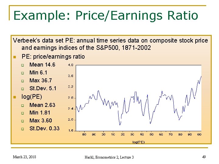
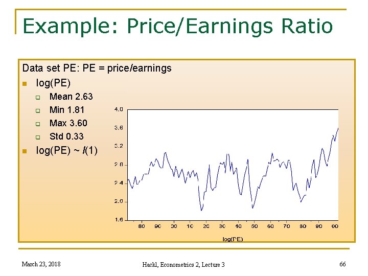
Example: Price/Earnings Ratio Verbeek’s data set PE: annual time series data on composite stock price and earnings indices of the S&P 500, 1871 -2002 n PE: price/earnings ratio q q n Mean 14. 6 Min 6. 1 Max 36. 7 St. Dev. 5. 1 log(PE) q q Mean 2. 63 Min 1. 81 Max 3. 60 St. Dev. 0. 33 March 23, 2018 Hackl, Econometrics 2, Lecture 3 49

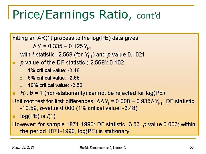
Price/Earnings Ratio, cont’d Fitting an AR(1) process to the log(PE) data gives: ΔYt = 0. 335 – 0. 125 Yt-1 with t-statistic -2. 569 (for Yt-1) and p-value 0. 1021 n p-value of the DF statistic (-2. 569): 0. 102 q q q 1% critical value: -3. 48 5% critical value: -2. 88 10% critical value: -2. 58 H 0: θ = 1 (non-stationarity) cannot be rejected for log(PE) Unit root test for first differences: ΔΔYt = 0. 008 – 0. 935ΔYt-1, DF statistic -10. 59, p-value 0. 000 (1% critical value: -3. 48) n log(PE) is I(1) However: for sample 1871 -1990: DF statistic -3. 65, p-value 0. 006; within the period 1871 -1990, log(PE) is stationary n March 23, 2018 Hackl, Econometrics 2, Lecture 3 50

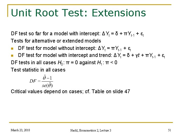
Unit Root Test: Extensions DF test so far for a model with intercept: ΔYt = δ + πYt-1 + εt Tests for alternative or extended models n DF test for model without intercept: ΔYt = πYt-1 + εt n DF test for model with intercept and trend: ΔYt = δ + γt + πYt-1 + εt DF tests in all cases H 0: π = 0 against H 1: π < 0 Test statistic in all cases Critical values depend on cases; cf. Table on slide 47 March 23, 2018 Hackl, Econometrics 2, Lecture 3 51

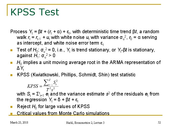
KPSS Test Process Yt = βt + (rt + α) + εt, with deterministic time trend βt, a random walk rt = rt-1 + ut with white noise ut with variance σu 2, r 0 = α serving as intercept, and white noise error term εt n Test of H 0: σu 2 = 0, i. e. , Yt is trend stationary, or Yt-βt is stationary, against H 1: σu 2 > 0 n H 0 implies a unit moving average root in the ARMA representation of ΔYt n KPSS (Kwiatkowski, Phillips, Schmidt, Shin) test statistic n n with St = Σti=1 ei and the variance estimate s 2 of the residuals et from the regression Yt = δ + βt + εt Reject H 0 for large values of KPSS Critical values from Monte Carlo simulations March 23, 2018 Hackl, Econometrics 2, Lecture 3 52

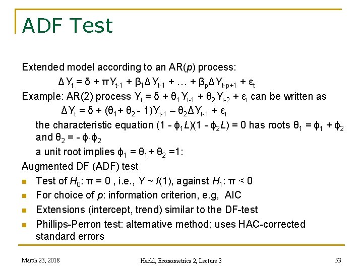
ADF Test Extended model according to an AR(p) process: ΔYt = δ + πYt-1 + β 1ΔYt-1 + … + βpΔYt-p+1 + εt Example: AR(2) process Yt = δ + θ 1 Yt-1 + θ 2 Yt-2 + εt can be written as ΔYt = δ + (θ 1+ θ 2 - 1)Yt-1 – θ 2ΔYt-1 + εt the characteristic equation (1 - ϕ 1 L)(1 - ϕ 2 L) = 0 has roots θ 1 = ϕ 1 + ϕ 2 and θ 2 = - ϕ 1ϕ 2 a unit root implies ϕ 1 = θ 1+ θ 2 =1: Augmented DF (ADF) test n Test of H 0: π = 0 , i. e. , Y ~ I(1), against H 1: π < 0 n For choice of p: information criterion, e. g, AIC n Extensions (intercept, trend) similar to the DF-test n Phillips-Perron test: alternative method; uses HAC-corrected standard errors March 23, 2018 Hackl, Econometrics 2, Lecture 3 53

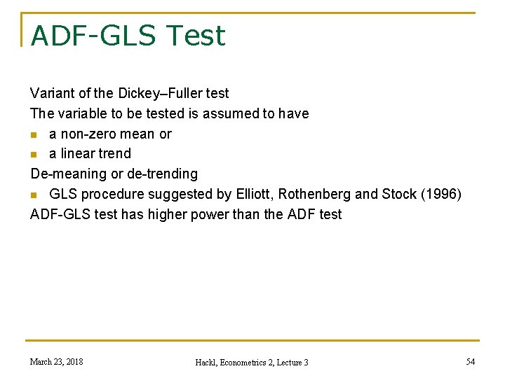
ADF-GLS Test Variant of the Dickey–Fuller test The variable to be tested is assumed to have n a non-zero mean or n a linear trend De-meaning or de-trending n GLS procedure suggested by Elliott, Rothenberg and Stock (1996) ADF-GLS test has higher power than the ADF test March 23, 2018 Hackl, Econometrics 2, Lecture 3 54

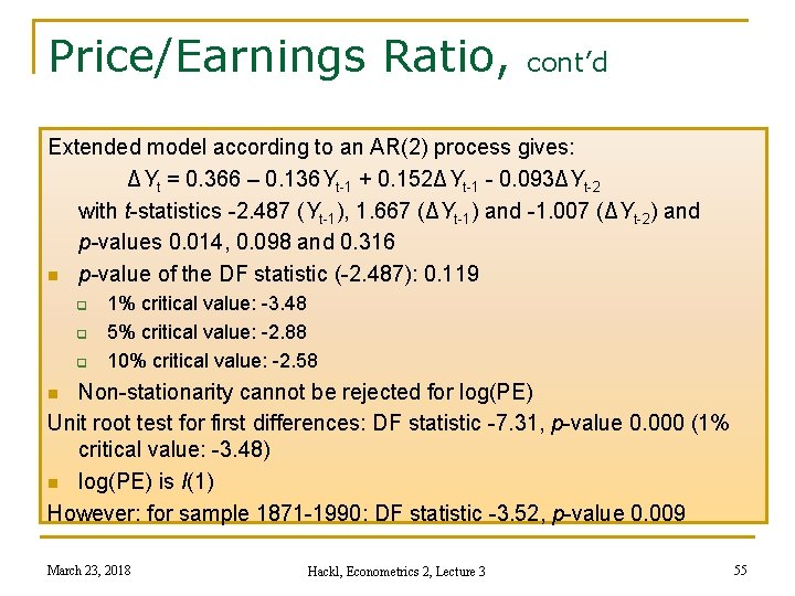
Price/Earnings Ratio, cont’d Extended model according to an AR(2) process gives: ΔYt = 0. 366 – 0. 136 Yt-1 + 0. 152ΔYt-1 - 0. 093ΔYt-2 with t-statistics -2. 487 (Yt-1), 1. 667 (ΔYt-1) and -1. 007 (ΔYt-2) and p-values 0. 014, 0. 098 and 0. 316 n p-value of the DF statistic (-2. 487): 0. 119 q q q 1% critical value: -3. 48 5% critical value: -2. 88 10% critical value: -2. 58 Non-stationarity cannot be rejected for log(PE) Unit root test for first differences: DF statistic -7. 31, p-value 0. 000 (1% critical value: -3. 48) n log(PE) is I(1) However: for sample 1871 -1990: DF statistic -3. 52, p-value 0. 009 n March 23, 2018 Hackl, Econometrics 2, Lecture 3 55

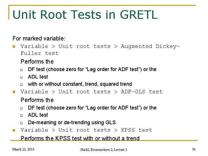
Unit Root Tests in GRETL For marked variable: n Variable > Unit root tests > Augmented Dickey. Fuller test Performs the q q q n Variable > Unit root tests > ADF-GLS test Performs the q q q n DF test (choose zero for “Lag order for ADF test”) or the ADL test with or without constant, trend, squared trend DF test (choose zero for “Lag order for ADF test”) or the ADL test De-meaning or de-trending using GLS Variable > Unit root tests > KPSS test Performs the KPSS test with or without a trend March 23, 2018 Hackl, Econometrics 2, Lecture 3 56

Contents n n n n Time Series Stochastic Processes Stationary Processes The ARMA Process Deterministic and Stochastic Trends Models with Trend Unit Root Tests Estimation of ARMA Models March 23, 2018 Hackl, Econometrics 2, Lecture 3 57

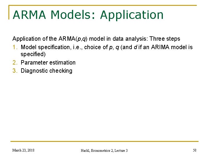
ARMA Models: Application of the ARMA(p, q) model in data analysis: Three steps 1. Model specification, i. e. , choice of p, q (and d if an ARIMA model is specified) 2. Parameter estimation 3. Diagnostic checking March 23, 2018 Hackl, Econometrics 2, Lecture 3 58

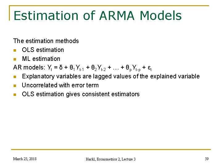
Estimation of ARMA Models The estimation methods n OLS estimation n ML estimation AR models: Yt = δ + θ 1 Yt-1 + θ 2 Yt-2 + … + θp. Yt-p + εt n Explanatory variables are lagged values of the explained variable n Uncorrelated with error term n OLS estimation gives consistent estimators March 23, 2018 Hackl, Econometrics 2, Lecture 3 59

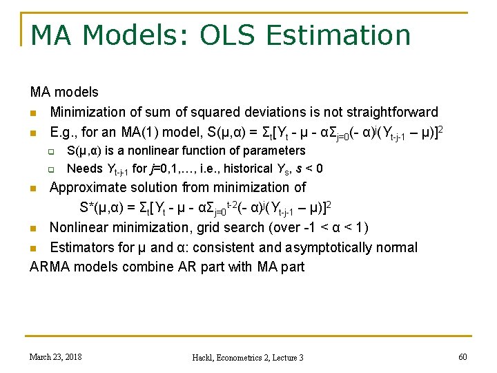
MA Models: OLS Estimation MA models n Minimization of sum of squared deviations is not straightforward n E. g. , for an MA(1) model, S(μ, α) = Σt[Yt - μ - αΣj=0(- α)j(Yt-j-1 – μ)]2 q q S(μ, α) is a nonlinear function of parameters Needs Yt-j-1 for j=0, 1, …, i. e. , historical Ys, s < 0 Approximate solution from minimization of S*(μ, α) = Σt[Yt - μ - αΣj=0 t-2(- α)j(Yt-j-1 – μ)]2 n Nonlinear minimization, grid search (over -1 < α < 1) n Estimators for μ and α: consistent and asymptotically normal ARMA models combine AR part with MA part n March 23, 2018 Hackl, Econometrics 2, Lecture 3 60

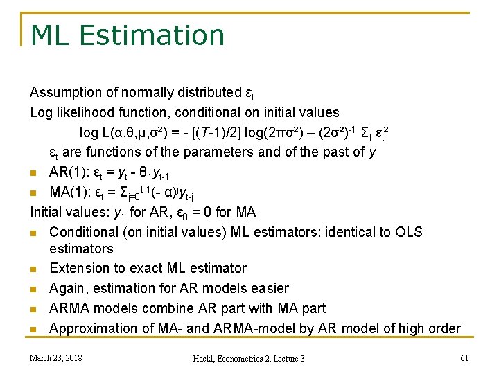
ML Estimation Assumption of normally distributed εt Log likelihood function, conditional on initial values log L(α, θ, μ, σ²) = - [(T-1)/2] log(2πσ²) – (2σ²)-1 Σt εt² εt are functions of the parameters and of the past of y n AR(1): εt = yt - θ 1 yt-1 n MA(1): εt = Σj=0 t-1(- α)jyt-j Initial values: y 1 for AR, ε 0 = 0 for MA n Conditional (on initial values) ML estimators: identical to OLS estimators n Extension to exact ML estimator n Again, estimation for AR models easier n ARMA models combine AR part with MA part n Approximation of MA- and ARMA-model by AR model of high order March 23, 2018 Hackl, Econometrics 2, Lecture 3 61

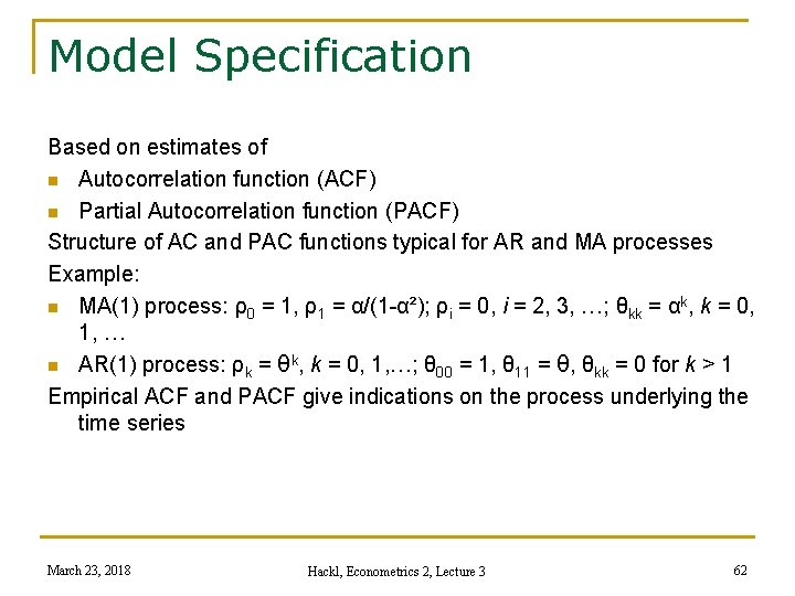
Model Specification Based on estimates of n Autocorrelation function (ACF) n Partial Autocorrelation function (PACF) Structure of AC and PAC functions typical for AR and MA processes Example: n MA(1) process: ρ0 = 1, ρ1 = α/(1 -α²); ρi = 0, i = 2, 3, …; θkk = αk, k = 0, 1, … n AR(1) process: ρk = θk, k = 0, 1, …; θ 00 = 1, θ 11 = θ, θkk = 0 for k > 1 Empirical ACF and PACF give indications on the process underlying the time series March 23, 2018 Hackl, Econometrics 2, Lecture 3 62

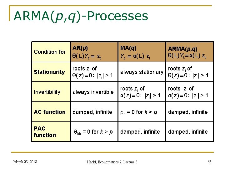
ARMA(p, q)-Processes Condition for AR(p) θ(L)Yt = εt Stationarity roots zi of always stationary θ(z)=0: |zi| > 1 Invertibility always invertible roots zi of α(z)=0: |zi| > 1 AC function damped, infinite rk = 0 for k > q damped, infinite PAC function θkk = 0 for k > p damped, infinite March 23, 2018 MA(q) Yt = α(L) εt Hackl, Econometrics 2, Lecture 3 ARMA(p, q) θ(L)Yt=α(L) εt 63

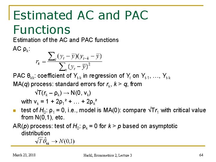
Estimated AC and PAC Functions Estimation of the AC and PAC functions AC ρk: PAC θkk: coefficient of Yt-k in regression of Yt on Yt-1, …, Yt-k MA(q) process: standard errors for rk, k > q, from √T(rk – ρk) → N(0, vk) with vk = 1 + 2ρ1² + … + 2ρk² n test of H 0: ρ1 = 0, i. e. , model is MA(0): compare √Tr 1 with critical value from N(0, 1), etc. AR(p) process: test of H 0: ρk = 0 for k > p based on asymptotic distribution March 23, 2018 Hackl, Econometrics 2, Lecture 3 64

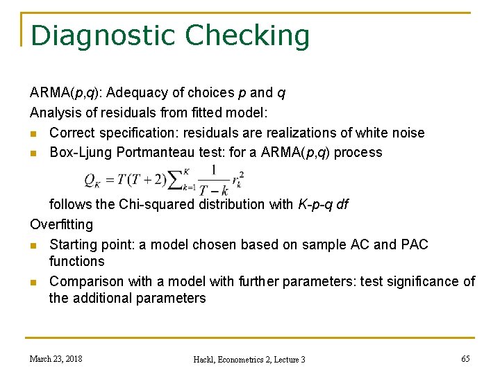
Diagnostic Checking ARMA(p, q): Adequacy of choices p and q Analysis of residuals from fitted model: n Correct specification: residuals are realizations of white noise n Box-Ljung Portmanteau test: for a ARMA(p, q) process follows the Chi-squared distribution with K-p-q df Overfitting n Starting point: a model chosen based on sample AC and PAC functions n Comparison with a model with further parameters: test significance of the additional parameters March 23, 2018 Hackl, Econometrics 2, Lecture 3 65

Example: Price/Earnings Ratio Data set PE: PE = price/earnings n log(PE) q q n Mean 2. 63 Min 1. 81 Max 3. 60 Std 0. 33 log(PE) ~ I(1) March 23, 2018 Hackl, Econometrics 2, Lecture 3 66

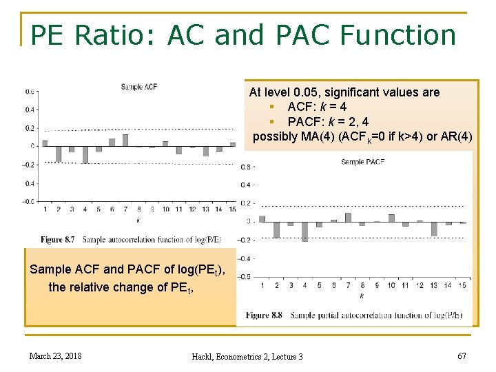
PE Ratio: AC and PAC Function At level 0. 05, significant values are § ACF: k = 4 § PACF: k = 2, 4 possibly MA(4) (ACFk=0 if k>4) or AR(4) Sample ACF and PACF of log(PEt), the relative change of PEt, March 23, 2018 Hackl, Econometrics 2, Lecture 3 67

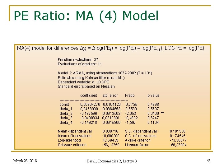
PE Ratio: MA (4) Model MA(4) model for differences Δyt = Δlog(PEt) = log(PEt) – log(PEt-1), LOGPE = log(PE) Function evaluations: 37 Evaluations of gradient: 11 Model 2: ARMA, using observations 1872 -2002 (T = 131) Estimated using Kalman filter (exact ML) Dependent variable: d_LOGPE Standard errors based on Hessian coefficient std. error t-ratio --------------------------- const 0, 00804276 0, 0104120 0, 7725 theta_1 0, 0478900 0, 0864653 0, 5539 theta_2 -0, 187566 0, 0913502 -2, 053 theta_3 -0, 0400834 0, 0819391 -0, 4892 theta_4 -0, 146218 0, 0915800 -1, 597 Mean dependent var Mean of innovations Log-likelihood Schwarz criterion March 23, 2018 0, 008716 -0, 000308 42, 69439 -56, 13759 p-value 0, 4398 0, 5797 0, 0400 ** 0, 6247 0, 1104 S. D. dependent var S. D. of innovations Akaike criterion Hannan-Quinn Hackl, Econometrics 2, Lecture 3 0, 181506 0, 174545 -73, 38877 -66, 37884 68

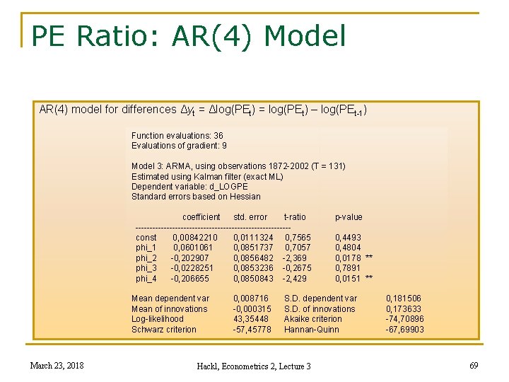
PE Ratio: AR(4) Model AR(4) model for differences Δyt = Δlog(PEt) = log(PEt) – log(PEt-1) Function evaluations: 36 Evaluations of gradient: 9 Model 3: ARMA, using observations 1872 -2002 (T = 131) Estimated using Kalman filter (exact ML) Dependent variable: d_LOGPE Standard errors based on Hessian coefficient std. error t-ratio --------------------------- const 0, 00842210 0, 0111324 0, 7565 phi_1 0, 0601061 0, 0851737 0, 7057 phi_2 -0, 202907 0, 0856482 -2, 369 phi_3 -0, 0228251 0, 0853236 -0, 2675 phi_4 -0, 206655 0, 0850843 -2, 429 Mean dependent var Mean of innovations Log-likelihood Schwarz criterion March 23, 2018 0, 008716 -0, 000315 43, 35448 -57, 45778 p-value 0, 4493 0, 4804 0, 0178 ** 0, 7891 0, 0151 ** S. D. dependent var S. D. of innovations Akaike criterion Hannan-Quinn Hackl, Econometrics 2, Lecture 3 0, 181506 0, 173633 -74, 70896 -67, 69903 69

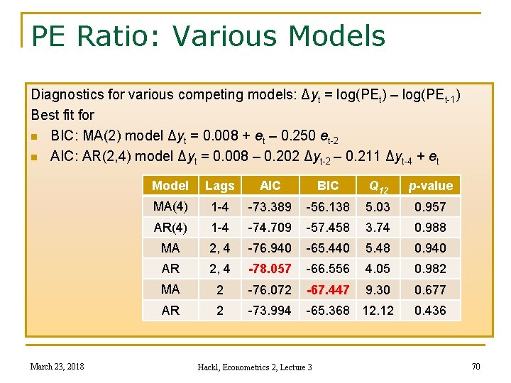
PE Ratio: Various Models Diagnostics for various competing models: Δyt = log(PEt) – log(PEt-1) Best fit for n BIC: MA(2) model Δyt = 0. 008 + et – 0. 250 et-2 n AIC: AR(2, 4) model Δyt = 0. 008 – 0. 202 Δyt-2 – 0. 211 Δyt-4 + et March 23, 2018 Model Lags AIC MA(4) 1 -4 -73. 389 -56. 138 5. 03 0. 957 AR(4) 1 -4 -74. 709 -57. 458 3. 74 0. 988 MA 2, 4 -76. 940 -65. 440 5. 48 0. 940 AR 2, 4 -78. 057 -66. 556 4. 05 0. 982 MA 2 -76. 072 -67. 447 9. 30 0. 677 AR 2 -73. 994 -65. 368 12. 12 0. 436 BIC Hackl, Econometrics 2, Lecture 3 Q 12 p-value 70

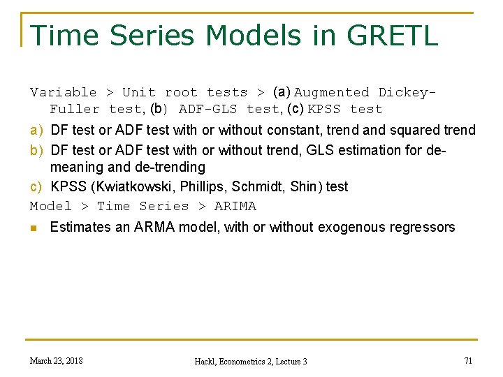
Time Series Models in GRETL Variable > Unit root tests > (a) Augmented Dickey. Fuller test, (b) ADF-GLS test, (c) KPSS test a) DF test or ADF test with or without constant, trend and squared trend b) DF test or ADF test with or without trend, GLS estimation for demeaning and de-trending c) KPSS (Kwiatkowski, Phillips, Schmidt, Shin) test Model > Time Series > ARIMA n Estimates an ARMA model, with or without exogenous regressors March 23, 2018 Hackl, Econometrics 2, Lecture 3 71

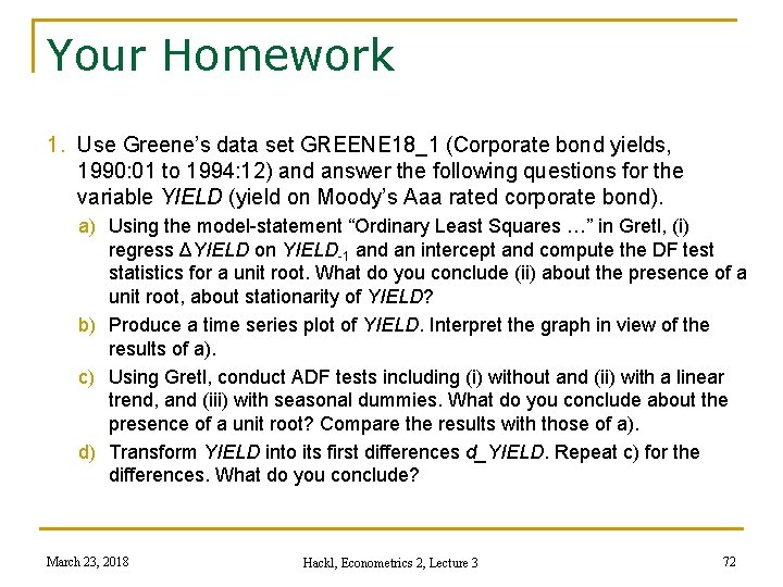
Your Homework 1. Use Greene’s data set GREENE 18_1 (Corporate bond yields, 1990: 01 to 1994: 12) and answer the following questions for the variable YIELD (yield on Moody’s Aaa rated corporate bond). a) Using the model-statement “Ordinary Least Squares …” in Gretl, (i) regress ΔYIELD on YIELD-1 and an intercept and compute the DF test statistics for a unit root. What do you conclude (ii) about the presence of a unit root, about stationarity of YIELD? b) Produce a time series plot of YIELD. Interpret the graph in view of the results of a). c) Using Gretl, conduct ADF tests including (i) without and (ii) with a linear trend, and (iii) with seasonal dummies. What do you conclude about the presence of a unit root? Compare the results with those of a). d) Transform YIELD into its first differences d_YIELD. Repeat c) for the differences. What do you conclude? March 23, 2018 Hackl, Econometrics 2, Lecture 3 72

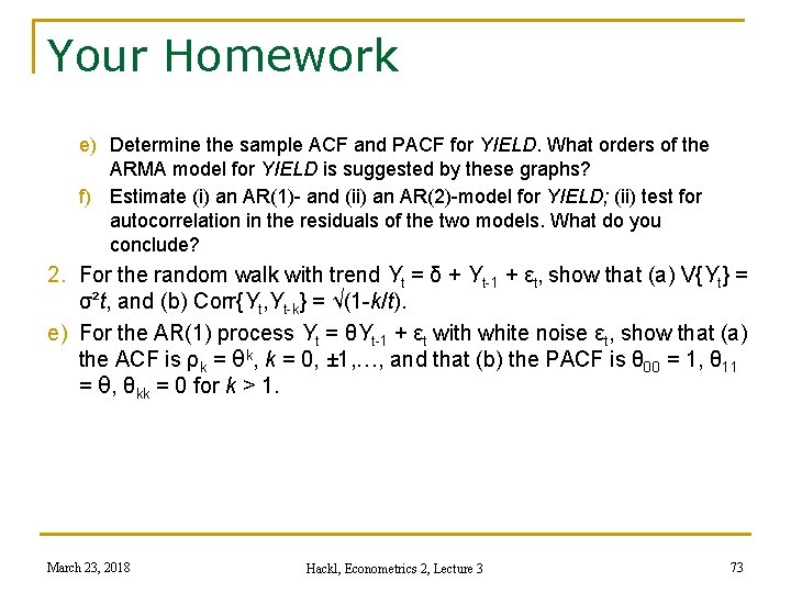
Your Homework e) Determine the sample ACF and PACF for YIELD. What orders of the ARMA model for YIELD is suggested by these graphs? f) Estimate (i) an AR(1)- and (ii) an AR(2)-model for YIELD; (ii) test for autocorrelation in the residuals of the two models. What do you conclude? 2. For the random walk with trend Yt = δ + Yt-1 + εt, show that (a) V{Yt} = σ²t, and (b) Corr{Yt, Yt-k} = √(1 -k/t). e) For the AR(1) process Yt = θYt-1 + εt with white noise εt, show that (a) the ACF is ρk = θk, k = 0, ± 1, …, and that (b) the PACF is θ 00 = 1, θ 11 = θ, θkk = 0 for k > 1. March 23, 2018 Hackl, Econometrics 2, Lecture 3 73