Econometrics 2 Lecture 1 ML Estimation Diagnostic Tests

Econometrics 2 - Lecture 1 ML Estimation, Diagnostic Tests

Contents n n Organizational Issues Linear Regression: A Review n Estimation of Regression Parameters Estimation Concepts ML Estimator: Idea and Illustrations ML Estimator: Notation and Properties ML Estimator: Two Examples Asymptotic Tests n Some Diagnostic Tests n n n Mar 11, 2016 Hackl, Econometrics 2, Lecture 1 2

Organizational Issues Course schedule (proposal) Class Date 1 Fr, Mar 11 2 Fr, Mar 18 3 Fr, Apr 1 4 Fr, Apr 15 5 Fr, Apr 22 6 Fr, Apr 29 Classes start at 10: 00 Mar 11, 2016 Hackl, Econometrics 2, Lecture 1 3

Organizational Issues, cont’d Teaching and learning method n Course in six blocks n Class discussion, written homework (computer exercises, GRETL) submitted by groups of (3 -5) students, presentations of homework by participants n Final exam Assessment of student work n For grading, the written homework, presentation of homework in class and a final written exam will be of relevance n Weights: homework 40 %, final written exam 60 % n Presentation of homework in class: students must be prepared to be called at random Mar 11, 2016 Hackl, Econometrics 2, Lecture 1 4

Organizational Issues, cont’d Literature Course textbook n Marno Verbeek, A Guide to Modern Econometrics, 3 rd Ed. , Wiley, 2008 Suggestions for further reading n W. H. Greene, Econometric Analysis. 7 th Ed. , Pearson International, 2012 n R. C. Hill, W. E. Griffiths, G. C. Lim, Principles of Econometrics, 4 th Ed. , Wiley, 2012 Mar 11, 2016 Hackl, Econometrics 2, Lecture 1 5

Aims and Content Aims of the course n Deepening the understanding of econometric concepts and principles n Learning about advanced econometric tools and techniques q q q n n ML estimation and testing methods (MV, Cpt. 6) Models for limited dependent variables (MV, Cpt. 7) Time series models (MV, Cpt. 8, 9) Multi-equation models (MV, Cpt. 9) Panel data models (MV, Cpt. 10) Use of econometric tools for analyzing economic data: specification of adequate models, identification of appropriate econometric methods, interpretation of results Use of GRETL Mar 11, 2016 Hackl, Econometrics 2, Lecture 1 6

Limited Dependent Variables: An Example Explain whether a household owns a car: explanatory power have n income n household size n etc. Regression is not suitable! WHY? Mar 11, 2016 Hackl, Econometrics 2, Lecture 1 7

Limited Dependent Variables: An Example Explain whether a household owns a car: explanatory power have n income n household size n etc. Regression is not suitable! n Owning a car has two manifestations: yes/no n Indicator for owning a car is a binary variable Models are needed that allow to describe a binary dependent variable or a, more generally, limited dependent variable Mar 11, 2016 Hackl, Econometrics 2, Lecture 1 8

Cases of Limited Dependent Variable Typical situations: functions of explanatory variables are used to describe or explain n Dichotomous dependent variable, e. g. , ownership of a car (yes/no), employment status (employed/unemployed), etc. n Ordered response, e. g. , qualitative assessment (good/average/bad), working status (full-time/part-time/not working), etc. n Multinomial response, e. g. , trading destinations (Europe/Asia/Africa), transportation means (train/bus/car), etc. n Count data, e. g. , number of orders a company receives in a week, number of patents granted to a company in a year n Censored data, e. g. , expenditures for durable goods, duration of study with drop outs Mar 11, 2016 Hackl, Econometrics 2, Lecture 1 9

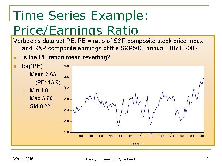
Time Series Example: Price/Earnings Ratio Verbeek’s data set PE: PE = ratio of S&P composite stock price index and S&P composite earnings of the S&P 500, annual, 1871 -2002 n Is the PE ration mean reverting? n log(PE) q q Mean 2. 63 (PE: 13, 9) Min 1. 81 Max 3. 60 Std 0. 33 Mar 11, 2016 Hackl, Econometrics 2, Lecture 1 10

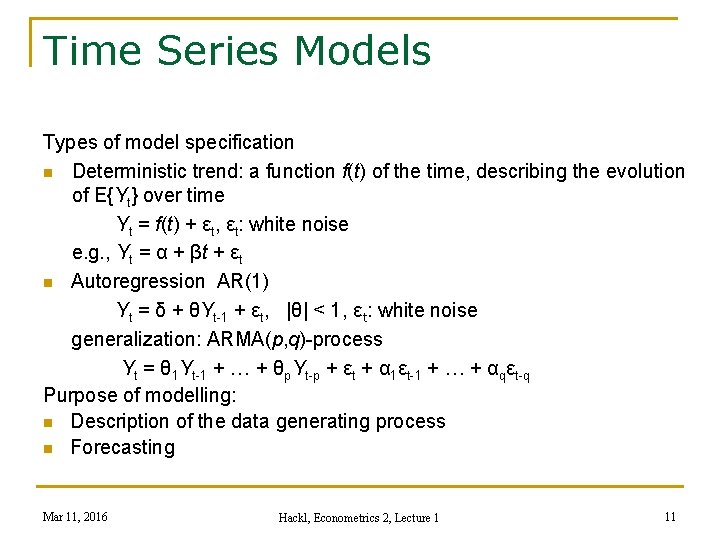
Time Series Models Types of model specification n Deterministic trend: a function f(t) of the time, describing the evolution of E{Yt} over time Yt = f(t) + εt, εt: white noise e. g. , Yt = α + βt + εt n Autoregression AR(1) Yt = δ + θYt-1 + εt, |θ| < 1, εt: white noise generalization: ARMA(p, q)-process Yt = θ 1 Yt-1 + … + θp. Yt-p + εt + α 1εt-1 + … + αqεt-q Purpose of modelling: n Description of the data generating process n Forecasting Mar 11, 2016 Hackl, Econometrics 2, Lecture 1 11

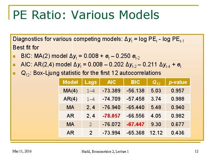
PE Ratio: Various Models Diagnostics for various competing models: Δyt = log PEt - log PEt-1 Best fit for n BIC: MA(2) model Δyt = 0. 008 + et – 0. 250 et-2 n AIC: AR(2, 4) model Δyt = 0. 008 – 0. 202 Δyt-2 – 0. 211 Δyt-4 + et n Q 12: Box-Ljung statistic for the first 12 autocorrelations Mar 11, 2016 Model Lags AIC BIC MA(4) 1 -4 -73. 389 -56. 138 5. 03 0. 957 AR(4) 1 -4 -74. 709 -57. 458 3. 74 0. 988 MA 2, 4 -76. 940 -65. 440 5. 48 0. 940 AR 2, 4 -78. 057 -66. 556 4. 05 0. 982 MA 2 -76. 072 -67. 447 9. 30 0. 677 AR 2 -73. 994 -65. 368 12. 12 0. 436 Hackl, Econometrics 2, Lecture 1 Q 12 p-value 12

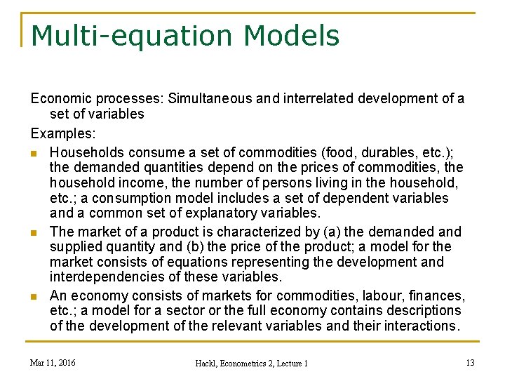
Multi-equation Models Economic processes: Simultaneous and interrelated development of a set of variables Examples: n Households consume a set of commodities (food, durables, etc. ); the demanded quantities depend on the prices of commodities, the household income, the number of persons living in the household, etc. ; a consumption model includes a set of dependent variables and a common set of explanatory variables. n The market of a product is characterized by (a) the demanded and supplied quantity and (b) the price of the product; a model for the market consists of equations representing the development and interdependencies of these variables. n An economy consists of markets for commodities, labour, finances, etc. ; a model for a sector or the full economy contains descriptions of the development of the relevant variables and their interactions. Mar 11, 2016 Hackl, Econometrics 2, Lecture 1 13

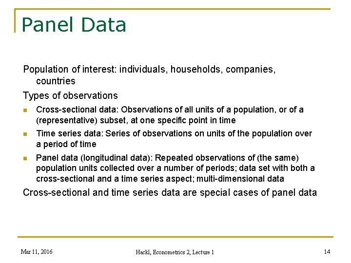
Panel Data Population of interest: individuals, households, companies, countries Types of observations n Cross-sectional data: Observations of all units of a population, or of a (representative) subset, at one specific point in time n Time series data: Series of observations on units of the population over a period of time n Panel data (longitudinal data): Repeated observations of (the same) population units collected over a number of periods; data set with both a cross-sectional and a time series aspect; multi-dimensional data Cross-sectional and time series data are special cases of panel data Mar 11, 2016 Hackl, Econometrics 2, Lecture 1 14

Panel Data Example: Individual Wages Verbeek’s data set “males” n Sample of q q n 545 full-time working males each person observed yearly after completion of school in 1980 till 1987 Variables q wage: log of hourly wage (in USD) q school: years of schooling q exper: age – 6 – school q q dummies for union membership, married, black, Hispanic, public sector others Mar 11, 2016 Hackl, Econometrics 2, Lecture 1 15

Panel Data Models Panel data models n Allow controlling individual differences, comparing behaviour, analysing dynamic adjustment, measuring effects of policy changes n More realistic models than cross-sectional and time-series models n Allow more detailed or sophisticated research questions E. g. : What is the effect of being married on the hourly wage Mar 11, 2016 Hackl, Econometrics 2, Lecture 1 16

Contents n n Organizational Issues Linear Regression: A Review n Estimation of Regression Parameters Estimation Concepts ML Estimator: Idea and Illustrations ML Estimator: Notation and Properties ML Estimator: Two Examples Asymptotic Tests n Some Diagnostic Tests n n n Mar 11, 2016 Hackl, Econometrics 2, Lecture 1 17

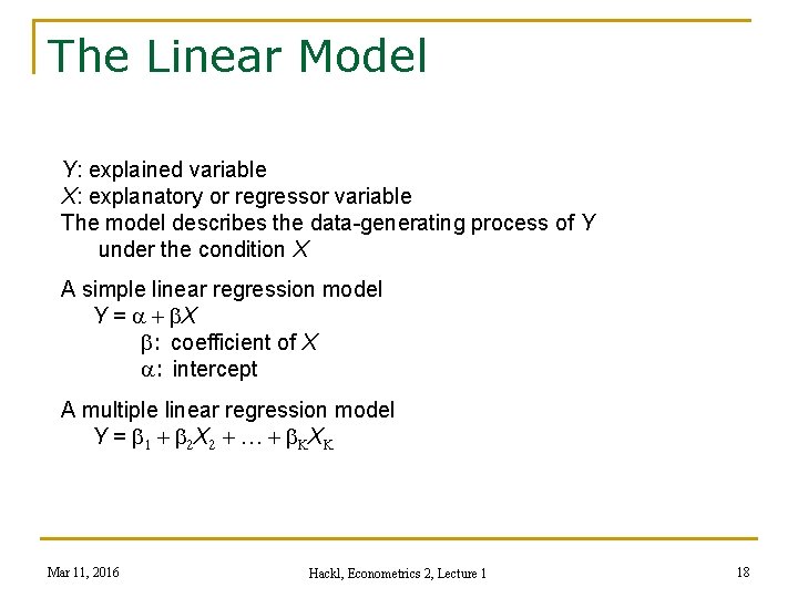
The Linear Model Y: explained variable X: explanatory or regressor variable The model describes the data-generating process of Y under the condition X A simple linear regression model Y = a + b. X b: coefficient of X a: intercept A multiple linear regression model Y = b 1 + b 2 X 2 + … + b. KXK Mar 11, 2016 Hackl, Econometrics 2, Lecture 1 18

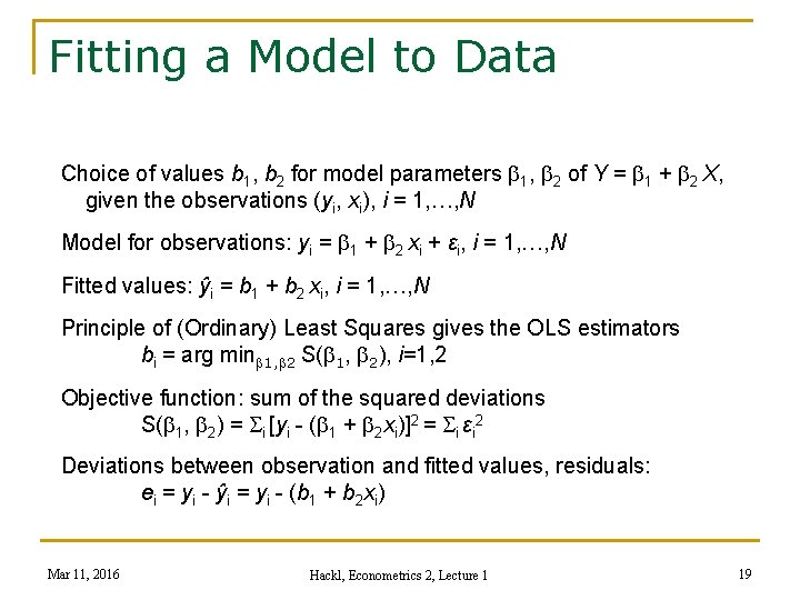
Fitting a Model to Data Choice of values b 1, b 2 for model parameters b 1, b 2 of Y = b 1 + b 2 X, given the observations (yi, xi), i = 1, …, N Model for observations: yi = b 1 + b 2 xi + εi, i = 1, …, N Fitted values: ŷi = b 1 + b 2 xi, i = 1, …, N Principle of (Ordinary) Least Squares gives the OLS estimators bi = arg minb 1, b 2 S(b 1, b 2), i=1, 2 Objective function: sum of the squared deviations S(b 1, b 2) = Si [yi - (b 1 + b 2 xi)]2 = Si εi 2 Deviations between observation and fitted values, residuals: ei = yi - ŷi = yi - (b 1 + b 2 xi) Mar 11, 2016 Hackl, Econometrics 2, Lecture 1 19

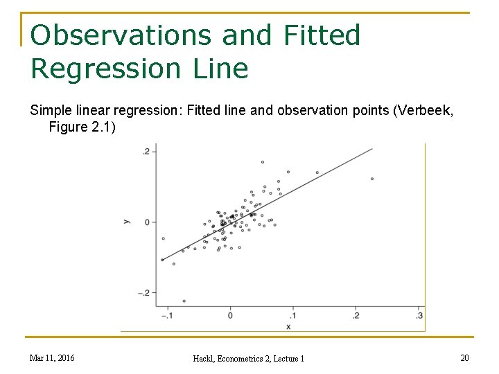
Observations and Fitted Regression Line Simple linear regression: Fitted line and observation points (Verbeek, Figure 2. 1) Mar 11, 2016 Hackl, Econometrics 2, Lecture 1 20

Contents n n Organizational Issues Linear Regression: A Review n Estimation of Regression Parameters Estimation Concepts ML Estimator: Idea and Illustrations ML Estimator: Notation and Properties ML Estimator: Two Examples Asymptotic Tests n Some Diagnostic Tests n n n Mar 11, 2016 Hackl, Econometrics 2, Lecture 1 21

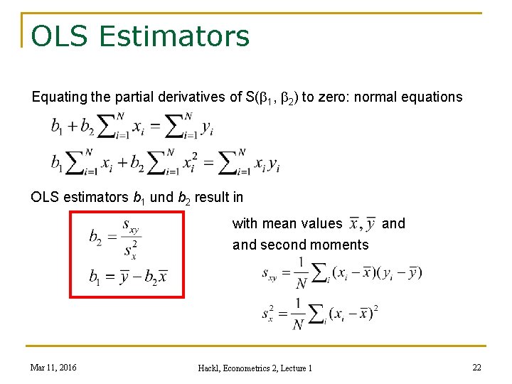
OLS Estimators Equating the partial derivatives of S(b 1, b 2) to zero: normal equations OLS estimators b 1 und b 2 result in with mean values and second moments Mar 11, 2016 Hackl, Econometrics 2, Lecture 1 22

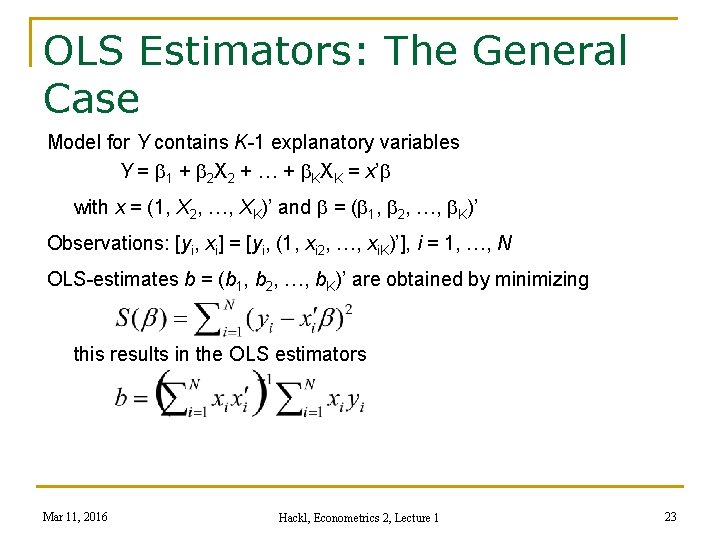
OLS Estimators: The General Case Model for Y contains K-1 explanatory variables Y = b 1 + b 2 X 2 + … + b. KXK = x’b with x = (1, X 2, …, XK)’ and b = (b 1, b 2, …, b. K)’ Observations: [yi, xi] = [yi, (1, xi 2, …, xi. K)’], i = 1, …, N OLS-estimates b = (b 1, b 2, …, b. K)’ are obtained by minimizing this results in the OLS estimators Mar 11, 2016 Hackl, Econometrics 2, Lecture 1 23

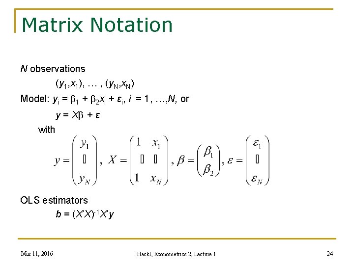
Matrix Notation N observations (y 1, x 1), … , (y. N, x. N) Model: yi = b 1 + b 2 xi + εi, i = 1, …, N, or y = Xb + ε with OLS estimators b = (X’X)-1 X’y Mar 11, 2016 Hackl, Econometrics 2, Lecture 1 24

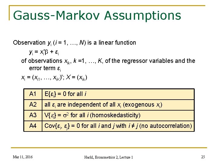
Gauss-Markov Assumptions Observation yi (i = 1, …, N) is a linear function yi = xi'b + εi of observations xik, k =1, …, K, of the regressor variables and the error term εi xi = (xi 1, …, xi. K)'; X = (xik) A 1 E{εi} = 0 for all i A 2 all εi are independent of all xi (exogenous xi) A 3 V{ei} = s 2 for all i (homoskedasticity) A 4 Cov{εi, εj} = 0 for all i and j with i ≠ j (no autocorrelation) Mar 11, 2016 Hackl, Econometrics 2, Lecture 1 25

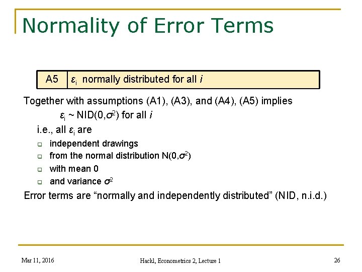
Normality of Error Terms A 5 εi normally distributed for all i Together with assumptions (A 1), (A 3), and (A 4), (A 5) implies εi ~ NID(0, σ2) for all i i. e. , all εi are q q independent drawings from the normal distribution N(0, σ2) with mean 0 and variance σ2 Error terms are “normally and independently distributed” (NID, n. i. d. ) Mar 11, 2016 Hackl, Econometrics 2, Lecture 1 26

Properties of OLS Estimators OLS estimator b = (X’X)-1 X’y 1. The OLS estimator b is unbiased: E{b} = β 2. The variance of the OLS estimator is given by V{b} = σ2(Σi xi xi’ )-1 3. The OLS estimator b is a BLUE (best linear unbiased estimator) for β 4. The OLS estimator b is normally distributed with mean β and covariance matrix V{b} = σ2(Σi xi xi’ )-1 Properties n 1. , 2. , and 3. follow from Gauss-Markov assumptions n 4. needs in addition the normality assumption (A 5) Mar 11, 2016 Hackl, Econometrics 2, Lecture 1 27

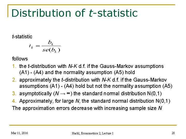
Distribution of t-statistic follows 1. the t-distribution with N-K d. f. if the Gauss-Markov assumptions (A 1) - (A 4) and the normality assumption (A 5) hold 2. approximately the t-distribution with N-K d. f. if the Gauss-Markov assumptions (A 1) - (A 4) hold but not the normality assumption (A 5) 3. asymptotically (N → ∞) the standard normal distribution N(0, 1) 4. Approximately, for large N, the standard normal distribution N(0, 1) The approximation errors decrease with increasing sample size N Mar 11, 2016 Hackl, Econometrics 2, Lecture 1 28

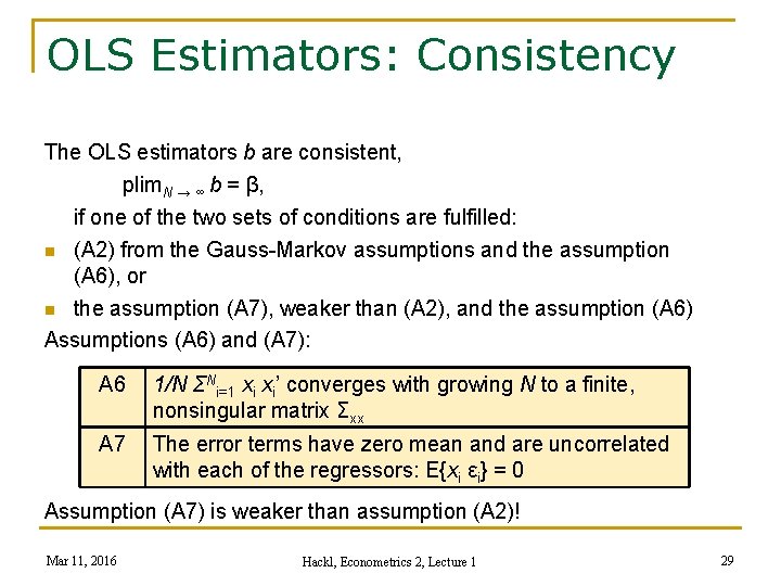
OLS Estimators: Consistency The OLS estimators b are consistent, plim. N → ∞ b = β, if one of the two sets of conditions are fulfilled: n (A 2) from the Gauss-Markov assumptions and the assumption (A 6), or n the assumption (A 7), weaker than (A 2), and the assumption (A 6) Assumptions (A 6) and (A 7): A 6 1/N ΣNi=1 xi xi’ converges with growing N to a finite, nonsingular matrix Σxx A 7 The error terms have zero mean and are uncorrelated with each of the regressors: E{xi εi} = 0 Assumption (A 7) is weaker than assumption (A 2)! Mar 11, 2016 Hackl, Econometrics 2, Lecture 1 29

Contents n n Organizational Issues Linear Regression: A Review n Estimation of Regression Parameters Estimation Concepts ML Estimator: Idea and Illustrations ML Estimator: Notation and Properties ML Estimator: Two Examples Asymptotic Tests n Some Diagnostic Tests n n n Mar 11, 2016 Hackl, Econometrics 2, Lecture 1 30

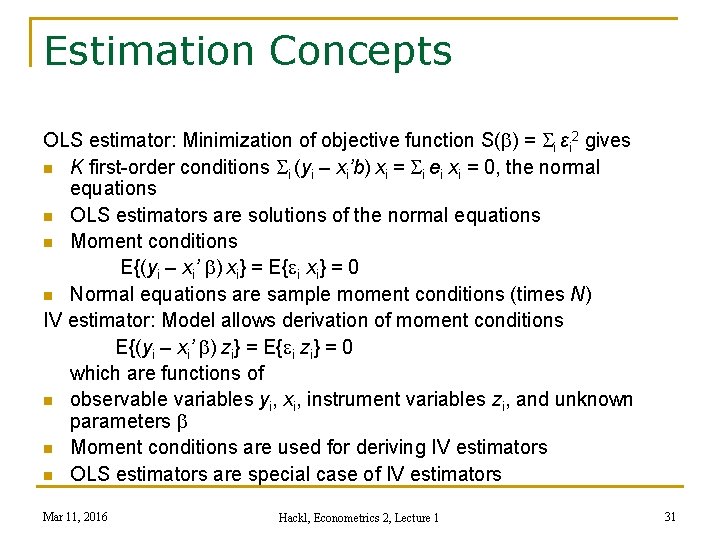
Estimation Concepts OLS estimator: Minimization of objective function S(b) = Si εi 2 gives n K first-order conditions Si (yi – xi’b) xi = Si ei xi = 0, the normal equations n OLS estimators are solutions of the normal equations n Moment conditions E{(yi – xi’ b) xi} = E{ei xi} = 0 n Normal equations are sample moment conditions (times N) IV estimator: Model allows derivation of moment conditions E{(yi – xi’ b) zi} = E{ei zi} = 0 which are functions of n observable variables yi, xi, instrument variables zi, and unknown parameters b n Moment conditions are used for deriving IV estimators n OLS estimators are special case of IV estimators Mar 11, 2016 Hackl, Econometrics 2, Lecture 1 31

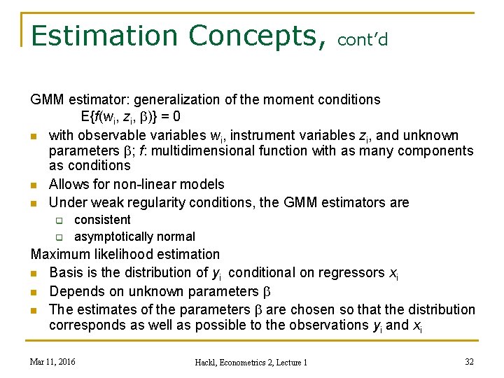
Estimation Concepts, cont’d GMM estimator: generalization of the moment conditions E{f(wi, zi, b)} = 0 n with observable variables wi, instrument variables zi, and unknown parameters b; f: multidimensional function with as many components as conditions n Allows for non-linear models n Under weak regularity conditions, the GMM estimators are q q consistent asymptotically normal Maximum likelihood estimation n Basis is the distribution of yi conditional on regressors xi n Depends on unknown parameters b n The estimates of the parameters b are chosen so that the distribution corresponds as well as possible to the observations yi and xi Mar 11, 2016 Hackl, Econometrics 2, Lecture 1 32

Contents n n Organizational Issues Linear Regression: A Review n Estimation of Regression Parameters Estimation Concepts ML Estimator: Idea and Illustrations ML Estimator: Notation and Properties ML Estimator: Two Examples Asymptotic Tests n Some Diagnostic Tests n n n Mar 11, 2016 Hackl, Econometrics 2, Lecture 1 33

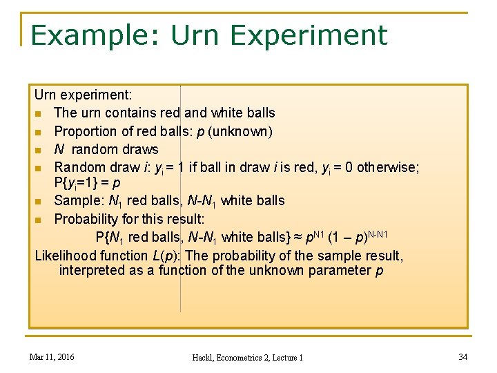
Example: Urn Experiment Urn experiment: n The urn contains red and white balls n Proportion of red balls: p (unknown) n N random draws n Random draw i: yi = 1 if ball in draw i is red, yi = 0 otherwise; P{yi=1} = p n Sample: N 1 red balls, N-N 1 white balls n Probability for this result: P{N 1 red balls, N-N 1 white balls} ≈ p. N 1 (1 – p)N-N 1 Likelihood function L(p): The probability of the sample result, interpreted as a function of the unknown parameter p Mar 11, 2016 Hackl, Econometrics 2, Lecture 1 34

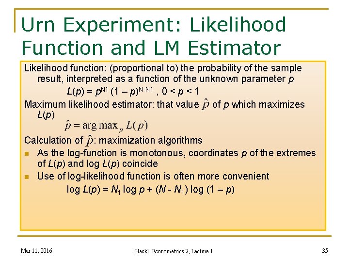
Urn Experiment: Likelihood Function and LM Estimator Likelihood function: (proportional to) the probability of the sample result, interpreted as a function of the unknown parameter p L(p) = p. N 1 (1 – p)N-N 1 , 0 < p < 1 Maximum likelihood estimator: that value of p which maximizes L(p) Calculation of : maximization algorithms n As the log-function is monotonous, coordinates p of the extremes of L(p) and log L(p) coincide n Use of log-likelihood function is often more convenient log L(p) = N 1 log p + (N - N 1) log (1 – p) Mar 11, 2016 Hackl, Econometrics 2, Lecture 1 35

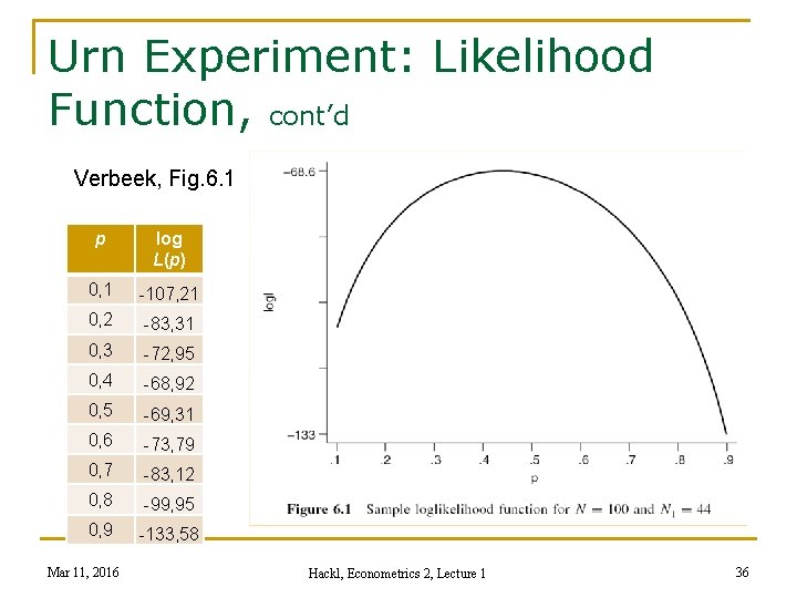
Urn Experiment: Likelihood Function, cont’d Verbeek, Fig. 6. 1 p log L(p) 0, 1 -107, 21 0, 2 -83, 31 0, 3 -72, 95 0, 4 -68, 92 0, 5 -69, 31 0, 6 -73, 79 0, 7 -83, 12 0, 8 -99, 95 0, 9 -133, 58 Mar 11, 2016 Hackl, Econometrics 2, Lecture 1 36

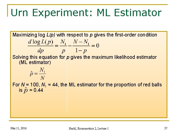
Urn Experiment: ML Estimator Maximizing log L(p) with respect to p gives the first-order condition Solving this equation for p gives the maximum likelihood estimator (ML estimator) For N = 100, N 1 = 44, the ML estimator for the proportion of red balls is = 0. 44 Mar 11, 2016 Hackl, Econometrics 2, Lecture 1 37

Maximum Likelihood Estimator: The Idea n n Specify the distribution of the data (of y or y given x) Determine the likelihood of observing the available sample as a function of the unknown parameters Choose as ML estimates those values for the unknown parameters that give the highest likelihood Properties: In general, the ML estimators are q consistent q asymptotically normal q efficient provided the likelihood function is correctly specified, i. e. , distributional assumptions are correct Mar 11, 2016 Hackl, Econometrics 2, Lecture 1 38

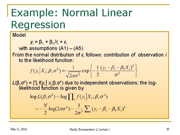
Example: Normal Linear Regression Model yi = β 1 + β 2 Xi + εi with assumptions (A 1) – (A 5) From the normal distribution of εi follows: contribution of observation i to the likelihood function: L(β, σ²) = ∏i f(yi│xi; β, σ²) due to independent observations; the loglikelihood function is given by Mar 11, 2016 Hackl, Econometrics 2, Lecture 1 39

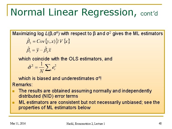
Normal Linear Regression, cont’d Maximizing log L(β, σ²) with respect to β and σ2 gives the ML estimators which coincide with the OLS estimators, and which is biased and underestimates σ²! Remarks: n The results are obtained assuming normally and independently distributed (NID) error terms n ML estimators are consistent but not necessarily unbiased; see the properties of ML estimators below Mar 11, 2016 Hackl, Econometrics 2, Lecture 1 40

Contents n n Organizational Issues Linear Regression: A Review n Estimation of Regression Parameters Estimation Concepts ML Estimator: Idea and Illustrations ML Estimator: Notation and Properties ML Estimator: Two Examples Asymptotic Tests n Some Diagnostic Tests n n n Mar 11, 2016 Hackl, Econometrics 2, Lecture 1 41

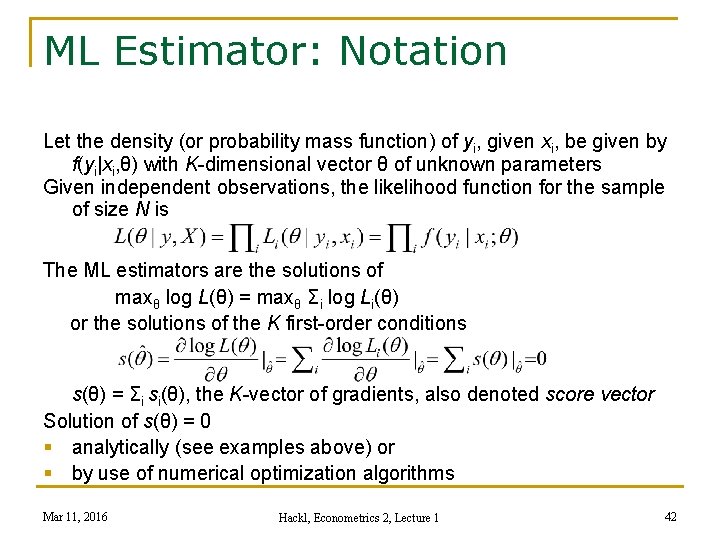
ML Estimator: Notation Let the density (or probability mass function) of yi, given xi, be given by f(yi|xi, θ) with K-dimensional vector θ of unknown parameters Given independent observations, the likelihood function for the sample of size N is The ML estimators are the solutions of maxθ log L(θ) = maxθ Σi log Li(θ) or the solutions of the K first-order conditions s(θ) = Σi si(θ), the K-vector of gradients, also denoted score vector Solution of s(θ) = 0 § analytically (see examples above) or § by use of numerical optimization algorithms Mar 11, 2016 Hackl, Econometrics 2, Lecture 1 42

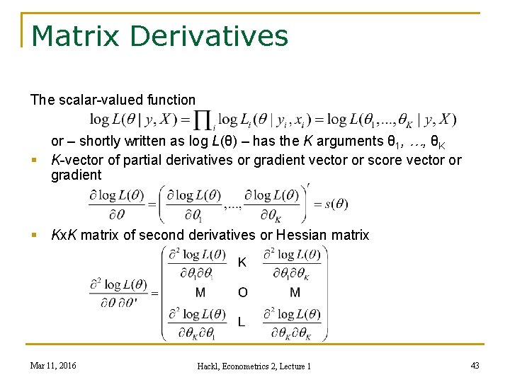
Matrix Derivatives The scalar-valued function or – shortly written as log L(θ) – has the K arguments θ 1, …, θK § K-vector of partial derivatives or gradient vector or score vector or gradient § Kx. K matrix of second derivatives or Hessian matrix Mar 11, 2016 Hackl, Econometrics 2, Lecture 1 43

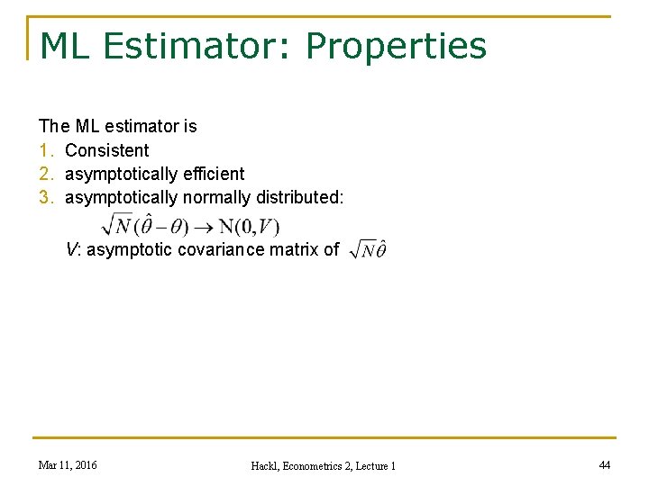
ML Estimator: Properties The ML estimator is 1. Consistent 2. asymptotically efficient 3. asymptotically normally distributed: V: asymptotic covariance matrix of Mar 11, 2016 Hackl, Econometrics 2, Lecture 1 44

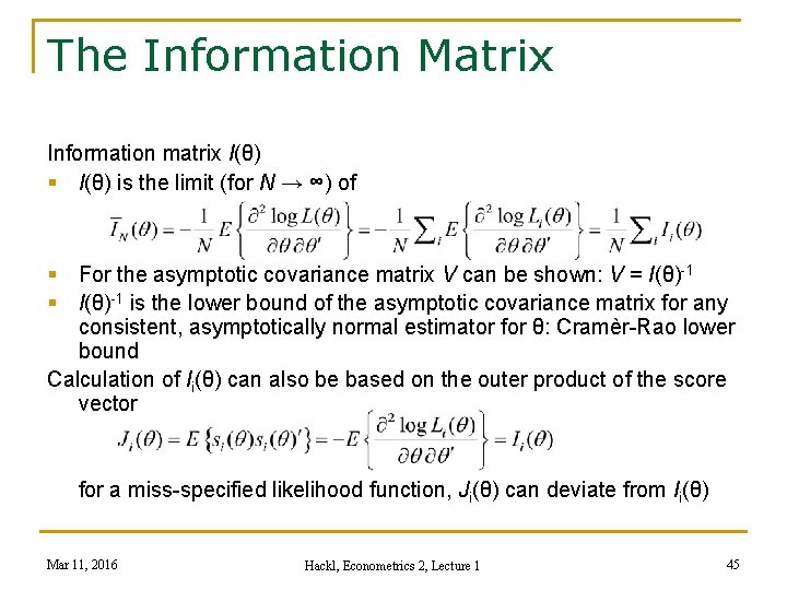
The Information Matrix Information matrix I(θ) § I(θ) is the limit (for N → ∞) of § For the asymptotic covariance matrix V can be shown: V = I(θ)-1 § I(θ)-1 is the lower bound of the asymptotic covariance matrix for any consistent, asymptotically normal estimator for θ: Cramèr-Rao lower bound Calculation of Ii(θ) can also be based on the outer product of the score vector for a miss-specified likelihood function, Ji(θ) can deviate from Ii(θ) Mar 11, 2016 Hackl, Econometrics 2, Lecture 1 45

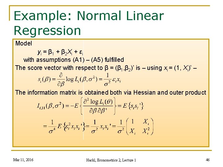
Example: Normal Linear Regression Model yi = β 1 + β 2 Xi + εi with assumptions (A 1) – (A 5) fulfilled The score vector with respect to β = (β 1, β 2)’ is – using xi = (1, Xi)’ – The information matrix is obtained both via Hessian and outer product Mar 11, 2016 Hackl, Econometrics 2, Lecture 1 46

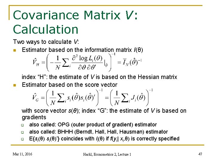
Covariance Matrix V: Calculation Two ways to calculate V: n Estimator based on the information matrix I(θ) n index “H”: the estimate of V is based on the Hessian matrix Estimator based on the score vector with score vector s(θ); index “G”: the estimate of V is based on gradients q q q also called: OPG (outer product of gradient) estimator also called: BHHH (Berndt, Hall, Hausman) estimator E{si(θ)’} coincides with Ii(θ) if f(yi| xi, θ) is correctly specified Mar 11, 2016 Hackl, Econometrics 2, Lecture 1 47

Contents n n Organizational Issues Linear Regression: A Review n Estimation of Regression Parameters Estimation Concepts ML Estimator: Idea and Illustrations ML Estimator: Notation and Properties ML Estimator: Two Examples Asymptotic Tests n Some Diagnostic Tests n n n Mar 11, 2016 Hackl, Econometrics 2, Lecture 1 48

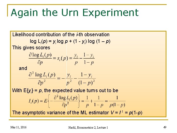
Again the Urn Experiment Likelihood contribution of the i-th observation log Li(p) = yi log p + (1 - yi) log (1 – p) This gives scores and With E{yi} = p, the expected value turns out to be The asymptotic variance of the ML estimator V = I-1 = p(1 -p) Mar 11, 2016 Hackl, Econometrics 2, Lecture 1 49

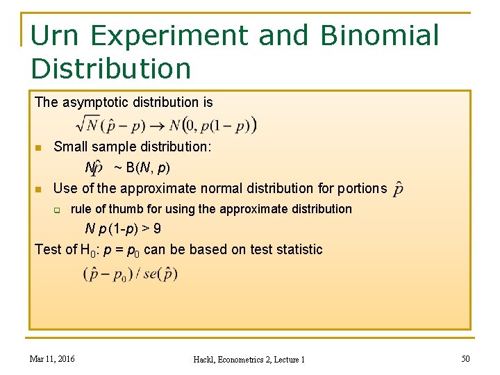
Urn Experiment and Binomial Distribution The asymptotic distribution is Small sample distribution: N ~ B(N, p) n Use of the approximate normal distribution for portions n q rule of thumb for using the approximate distribution N p (1 -p) > 9 Test of H 0: p = p 0 can be based on test statistic Mar 11, 2016 Hackl, Econometrics 2, Lecture 1 50

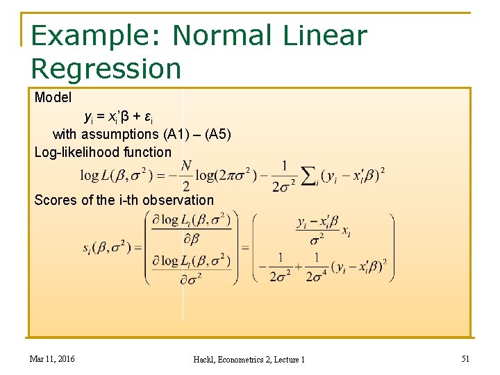
Example: Normal Linear Regression Model yi = xi’β + εi with assumptions (A 1) – (A 5) Log-likelihood function Scores of the i-th observation Mar 11, 2016 Hackl, Econometrics 2, Lecture 1 51

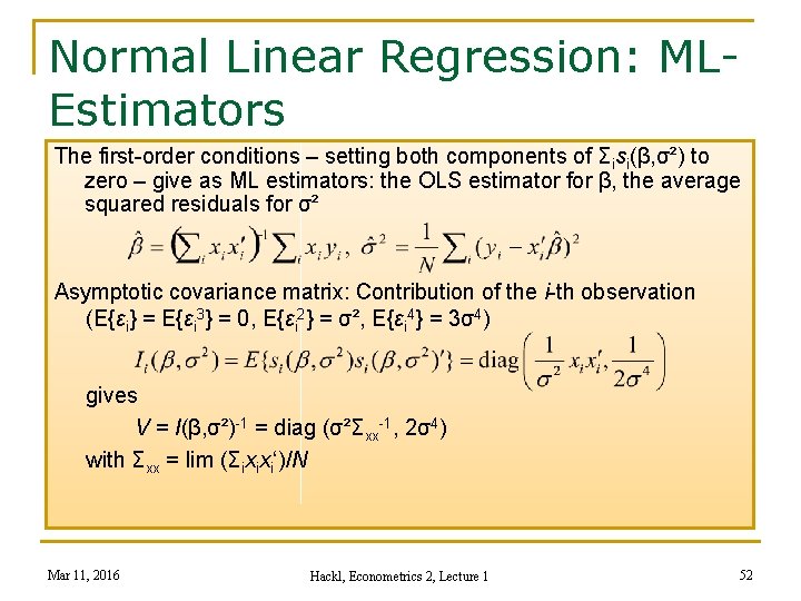
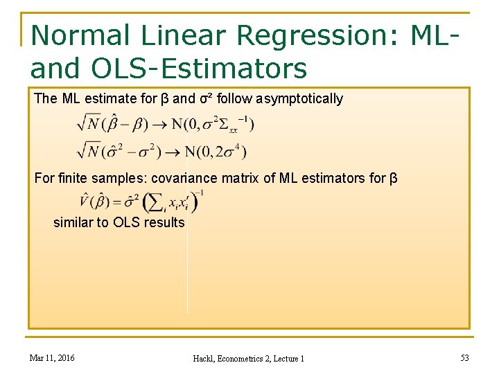
Normal Linear Regression: MLEstimators The first-order conditions – setting both components of Σisi(β, σ²) to zero – give as ML estimators: the OLS estimator for β, the average squared residuals for σ² Asymptotic covariance matrix: Contribution of the i-th observation (E{εi} = E{εi 3} = 0, E{εi 2} = σ², E{εi 4} = 3σ4) gives V = I(β, σ²)-1 = diag (σ²Σxx-1, 2σ4) with Σxx = lim (Σixixi‘)/N Mar 11, 2016 Hackl, Econometrics 2, Lecture 1 52

Normal Linear Regression: MLand OLS-Estimators The ML estimate for β and σ² follow asymptotically For finite samples: covariance matrix of ML estimators for β similar to OLS results Mar 11, 2016 Hackl, Econometrics 2, Lecture 1 53

Contents n n Organizational Issues Linear Regression: A Review n Estimation of Regression Parameters Estimation Concepts ML Estimator: Idea and Illustrations ML Estimator: Notation and Properties ML Estimator: Two Examples Asymptotic Tests n Some Diagnostic Tests n n n Mar 11, 2016 Hackl, Econometrics 2, Lecture 1 54

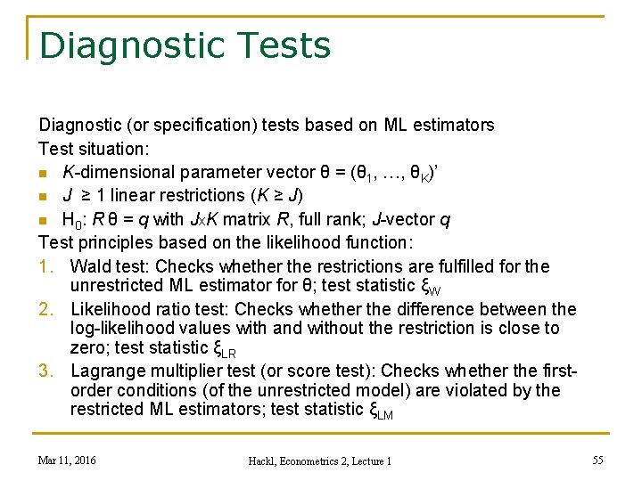
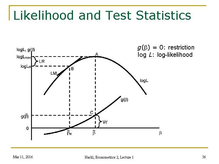
Diagnostic Tests Diagnostic (or specification) tests based on ML estimators Test situation: n K-dimensional parameter vector θ = (θ 1, …, θK)’ n J ≥ 1 linear restrictions (K ≥ J) n H 0: R θ = q with Jx. K matrix R, full rank; J-vector q Test principles based on the likelihood function: 1. Wald test: Checks whether the restrictions are fulfilled for the unrestricted ML estimator for θ; test statistic ξW 2. Likelihood ratio test: Checks whether the difference between the log-likelihood values with and without the restriction is close to zero; test statistic ξLR 3. Lagrange multiplier test (or score test): Checks whether the firstorder conditions (of the unrestricted model) are violated by the restricted ML estimators; test statistic ξLM Mar 11, 2016 Hackl, Econometrics 2, Lecture 1 55

Likelihood and Test Statistics g(b) = 0: restriction log L: log-likelihood Mar 11, 2016 Hackl, Econometrics 2, Lecture 1 56

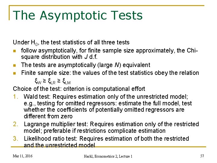
The Asymptotic Tests Under H 0, the test statistics of all three tests n follow asymptotically, for finite sample size approximately, the Chisquare distribution with J d. f. n The tests are asymptotically (large N) equivalent n Finite sample size: the values of the test statistics obey the relation ξW ≥ ξLR ≥ ξLM Choice of the test: criterion is computational effort 1. Wald test: Requires estimation only of the unrestricted model; e. g. , testing for omitted regressors: estimate the full model, test whether the coefficients of potentially omitted regressors are different from zero 2. Lagrange multiplier test: Requires estimation only of the restricted model; preferable if restrictions complicate estimation 3. Likelihood ratio test: Requires estimation of both the restricted and the unrestricted model Mar 11, 2016 Hackl, Econometrics 2, Lecture 1 57

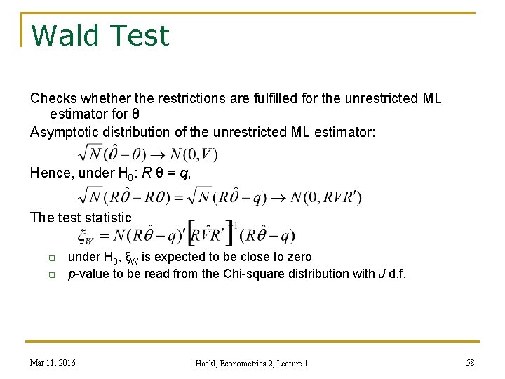
Wald Test Checks whether the restrictions are fulfilled for the unrestricted ML estimator for θ Asymptotic distribution of the unrestricted ML estimator: Hence, under H 0: R θ = q, The test statistic q q under H 0, ξW is expected to be close to zero p-value to be read from the Chi-square distribution with J d. f. Mar 11, 2016 Hackl, Econometrics 2, Lecture 1 58

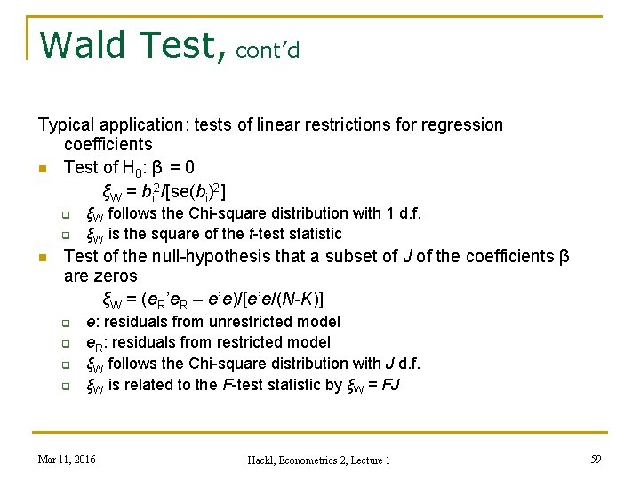
Wald Test, cont’d Typical application: tests of linear restrictions for regression coefficients n Test of H 0: βi = 0 ξW = bi 2/[se(bi)2] q q n ξW follows the Chi-square distribution with 1 d. f. ξW is the square of the t-test statistic Test of the null-hypothesis that a subset of J of the coefficients β are zeros ξW = (e. R’e. R – e’e)/[e’e/(N-K)] q q e: residuals from unrestricted model e. R: residuals from restricted model ξW follows the Chi-square distribution with J d. f. ξW is related to the F-test statistic by ξW = FJ Mar 11, 2016 Hackl, Econometrics 2, Lecture 1 59

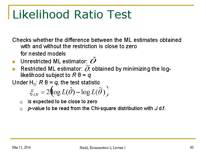
Likelihood Ratio Test Checks whether the difference between the ML estimates obtained with and without the restriction is close to zero for nested models n Unrestricted ML estimator: n Restricted ML estimator: ; obtained by minimizing the loglikelihood subject to R θ = q Under H 0: R θ = q, the test statistic q q is expected to be close to zero p-value to be read from the Chi-square distribution with J d. f. Mar 11, 2016 Hackl, Econometrics 2, Lecture 1 60

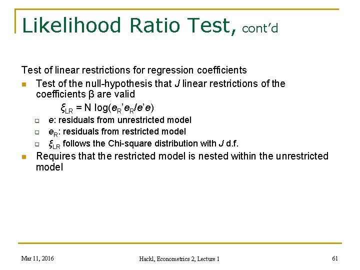
Likelihood Ratio Test, cont’d Test of linear restrictions for regression coefficients n Test of the null-hypothesis that J linear restrictions of the coefficients β are valid ξLR = N log(e. R’e. R/e’e) q q q n e: residuals from unrestricted model e. R: residuals from restricted model ξLR follows the Chi-square distribution with J d. f. Requires that the restricted model is nested within the unrestricted model Mar 11, 2016 Hackl, Econometrics 2, Lecture 1 61

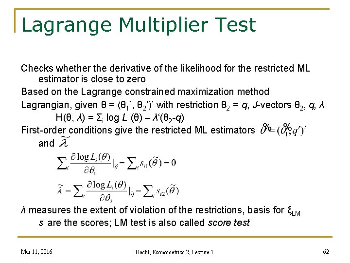
Lagrange Multiplier Test Checks whether the derivative of the likelihood for the restricted ML estimator is close to zero Based on the Lagrange constrained maximization method Lagrangian, given θ = (θ 1’, θ 2’)’ with restriction θ 2 = q, J-vectors θ 2, q, λ H(θ, λ) = Σi log L i(θ) – λ‘(θ 2 -q) First-order conditions give the restricted ML estimators and λ measures the extent of violation of the restrictions, basis for ξLM si are the scores; LM test is also called score test Mar 11, 2016 Hackl, Econometrics 2, Lecture 1 62

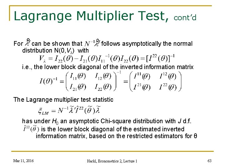
Lagrange Multiplier Test, cont’d For can be shown that follows asymptotically the normal distribution N(0, Vλ) with i. e. , the lower block diagonal of the inverted information matrix The Lagrange multiplier test statistic has under H 0 an asymptotic Chi-square distribution with J d. f. is the lower block diagonal of the estimated inverted information matrix, based on the restricted estimators for θ Mar 11, 2016 Hackl, Econometrics 2, Lecture 1 63

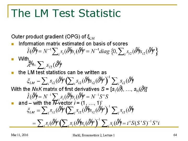
The LM Test Statistic Outer product gradient (OPG) of ξLM n Information matrix estimated on basis of scores n With n the LM test statistics can be written as With the Nx. K matrix of first derivatives S = [s 1( ), …, s. N( )]‘ n and – with the N-vector i = (1, …, 1)’ Mar 11, 2016 Hackl, Econometrics 2, Lecture 1 64

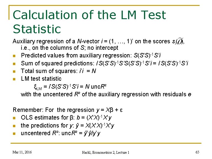
Calculation of the LM Test Statistic Auxiliary regression of a N-vector i = (1, …, 1)’ on the scores si( ), i. e. , on the columns of S; no intercept n Predicted values from auxiliary regression: S(S'S)-1 S’i n Sum of squared predictions: i’S(S’S)-1 S’i = i’S(S’S)-1 S’i n Total sum of squares: i’i = N n LM test statistic ξLM = i’S(S’S)-1 S’i = N unc. R² with the uncentered R² of the auxiliary regression with residuals e Remember: For the regression y = Xβ + ε n OLS estimates for β: b = (X‘X)-1 X‘y n the predictions for y: ŷ = X(X‘X)-1 X‘y n uncentered R²: unc. R² = ŷ’ŷ/y’y Mar 11, 2016 Hackl, Econometrics 2, Lecture 1 65

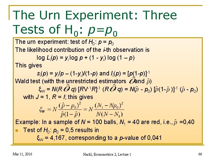
The Urn Experiment: Three Tests of H 0: p=p 0 The urn experiment: test of H 0: p = p 0 The likelihood contribution of the i-th observation is log Li(p) = yi log p + (1 - yi) log (1 – p) This gives si(p) = yi/p – (1 -yi)/(1 -p) and Ii(p) = [p(1 -p)]-1 Wald test (with the unrestricted estimators and ) ξW = N(R - q) [RV-1 R]-1 (R - q) = N( - p 0) [ (1 - )]-1 ( - p 0) with J = 1, R = I; this gives Example: In a sample of N = 100 balls, N 1 = 40 are red, i. e. , =0, 40 n Test of H 0: p 0 = 0, 5 results in ξW = 4, 167, corresponding to a p-value of 0, 041 Mar 11, 2016 Hackl, Econometrics 2, Lecture 1 66

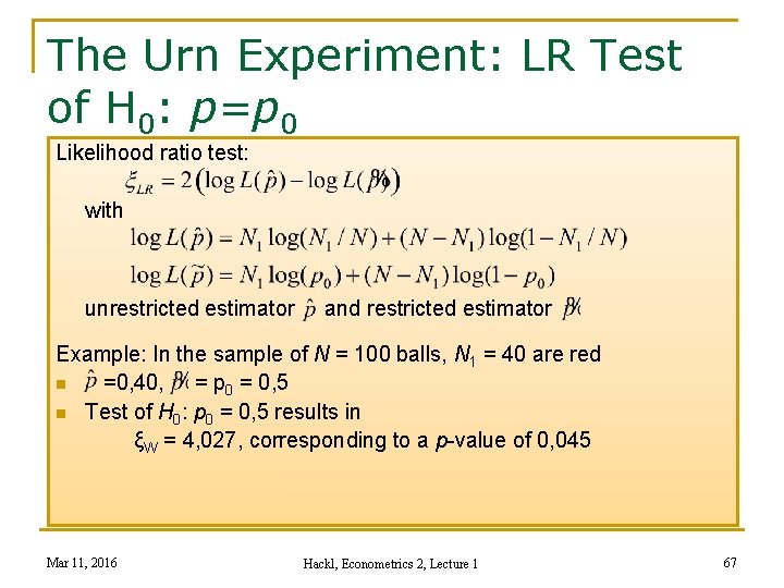
The Urn Experiment: LR Test of H 0: p=p 0 Likelihood ratio test: with unrestricted estimator and restricted estimator Example: In the sample of N = 100 balls, N 1 = 40 are red n =0, 40, = p 0 = 0, 5 n Test of H 0: p 0 = 0, 5 results in ξW = 4, 027, corresponding to a p-value of 0, 045 Mar 11, 2016 Hackl, Econometrics 2, Lecture 1 67

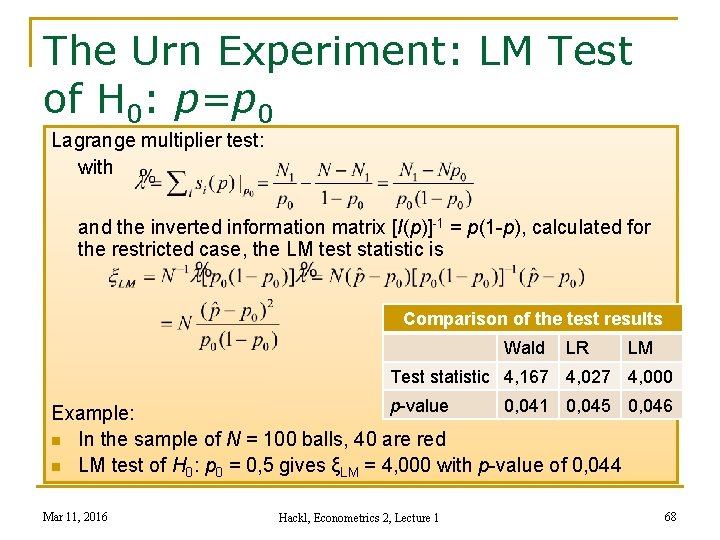
The Urn Experiment: LM Test of H 0: p=p 0 Lagrange multiplier test: with and the inverted information matrix [I(p)]-1 = p(1 -p), calculated for the restricted case, the LM test statistic is Comparison of the test results Wald LR LM Test statistic 4, 167 4, 027 4, 000 p-value 0, 041 0, 045 0, 046 Example: n In the sample of N = 100 balls, 40 are red n LM test of H 0: p 0 = 0, 5 gives ξLM = 4, 000 with p-value of 0, 044 Mar 11, 2016 Hackl, Econometrics 2, Lecture 1 68

Contents n n Organizational Issues Linear Regression: A Review n Estimation of Regression Parameters Estimation Concepts ML Estimator: Idea and Illustrations ML Estimator: Notation and Properties ML Estimator: Two Examples Asymptotic Tests n Some Diagnostic Tests n n n Mar 11, 2016 Hackl, Econometrics 2, Lecture 1 69

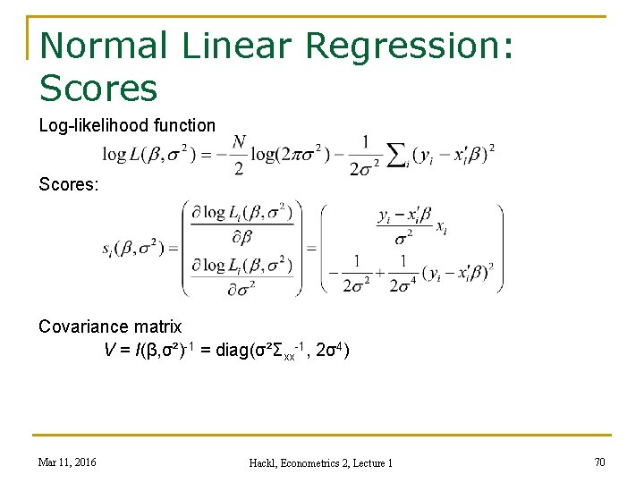
Normal Linear Regression: Scores Log-likelihood function Scores: Covariance matrix V = I(β, σ²)-1 = diag(σ²Σxx-1, 2σ4) Mar 11, 2016 Hackl, Econometrics 2, Lecture 1 70

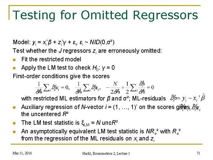
Testing for Omitted Regressors Model: yi = xi’β + zi’γ + εi, εi ~ NID(0, σ²) Test whether the J regressors zi are erroneously omitted: n Fit the restricted model n Apply the LM test to check H 0: γ = 0 First-order conditions give the scores n n n with restricted ML estimators for β and σ²; ML-residuals Auxiliary regression of N-vector i = (1, …, 1)’ on the scores gives the uncentered R² The LM test statistic is ξLM = N unc. R² An asymptotically equivalent LM test statistic is NRe² with Re² from the regression of the ML residuals on xi and zi Mar 11, 2016 Hackl, Econometrics 2, Lecture 1 71

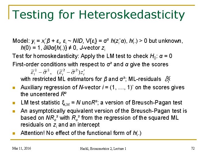
Testing for Heteroskedasticity Model: yi = xi’β + εi, εi ~ NID, V{εi} = σ² h(zi’α), h(. ) > 0 but unknown, h(0) = 1, ∂/∂α{h(. )} ≠ 0, J-vector zi Test for homoskedasticity: Apply the LM test to check H 0: α = 0 First-order conditions with respect to σ² and α give the scores n n with restricted ML estimators for β and σ²; ML-residuals Auxiliary regression of N-vector i = (1, …, 1)’ on the scores gives the uncentered R² LM test statistic ξLM = N unc. R²; a version of Breusch-Pagan test An asymptotically equivalent version of the Breusch-Pagan test is based on NRe² with Re² from the regression of the squared ML residuals on zi and an intercept Attention! No effect of the functional form of h(. ) Mar 11, 2016 Hackl, Econometrics 2, Lecture 1 72

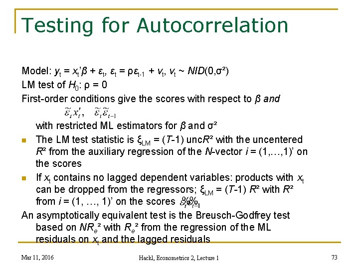
Testing for Autocorrelation Model: yt = xt’β + εt, εt = ρεt-1 + vt, vt ~ NID(0, σ²) LM test of H 0: ρ = 0 First-order conditions give the scores with respect to β and with restricted ML estimators for β and σ² n The LM test statistic is ξLM = (T-1) unc. R² with the uncentered R² from the auxiliary regression of the N-vector i = (1, …, 1)’ on the scores n If xt contains no lagged dependent variables: products with xt can be dropped from the regressors; ξLM = (T-1) R² with R² from i = (1, …, 1)’ on the scores An asymptotically equivalent test is the Breusch-Godfrey test based on NRe² with Re² from the regression of the ML residuals on xt and the lagged residuals Mar 11, 2016 Hackl, Econometrics 2, Lecture 1 73

Your Homework 1. Assume that the errors εt of the linear regression yt = β 1 + β 2 xt + εt are NID(0, σ2) distributed. (a) Determine the log-likelihood function of the sample for t = 1, …, T; (b) derive (i) the first-order conditions and (ii) the ML estimators for β 1, β 2, and σ2; (c) derive the asymptotic covariance matrix of the ML estimators for β 1 and β 2 on the basis (i) of the information matrix and (ii) of the score vector. 2. Open the Greene sample file “greene 7_8, Gasoline price and consumption”, offered within the Gretl system. The dataset contains time series of annual observations from 1960 through 1995. The variables to be used in the following are: G = total U. S. gasoline consumption, computed as total expenditure of gas divided by the price index; Pg = price index for gasoline; Y = per capita disposable income; Pnc = price index for new cars; Mar 11, 2016 Hackl, Econometrics 2, Lecture 1 74

Your Homework, cont’d Puc = price index for used cars; Pop = U. S. total population in millions. Perform the following analyses and interpret the results: a. Produce and interpret the scatter plot of the per capita (p. c. ) gasoline consumption (Gpc) over the p. c. disposable income (Y). b. Fit the linear regression for log(Gpc) with regressors log(Y), Pg, Pnc and Puc to the data and give an interpretation of the outcome. c. Use the Chow test to test for a structural break between 1979 and 1980. d. Test for autocorrelation of the error terms using the LM test statistic ξLM = (T-1) R² with R² from the auxiliary regression of the vector of ones i = (1, …, 1)’ on the scores (et*et-1). e. Test for autocorrelation by means of the Breusch-Godfrey test, using the test statistic TRe² with Re² from the regression of the residuals on the regressors and the lagged residuals. Mar 11, 2016 Hackl, Econometrics 2, Lecture 1 75