Econometric methods of analysis and forecasting of financial
- Slides: 17

Econometric methods of analysis and forecasting of financial markets Lecture 3. Time series modeling and forecasting

From this lecture you will learn: • How to make the forecast for autoregressive moving average (ARMA) models and exponential smoothing models • How to estimate the accuracy of predictions with the use of different metrics • How to estimate time series models and make the forecasts in EViews

Contents: • • The nature of time series AR, MA, ARMA models Box–Jenkins methodology ARCH-and GARCH-models Stationarity Unit roots Examples of time series modelling in finance

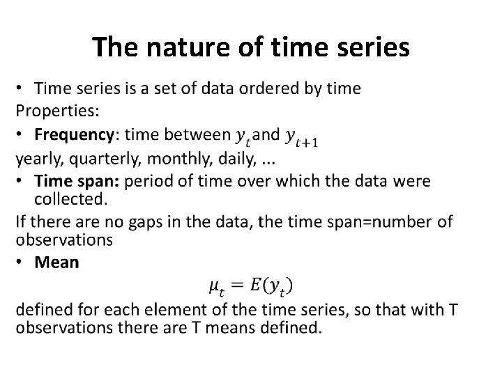
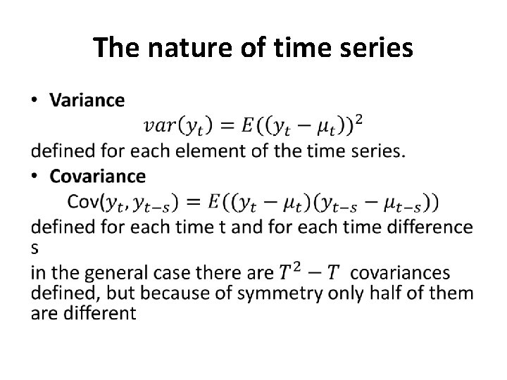
The nature of time series •

The nature of time series •

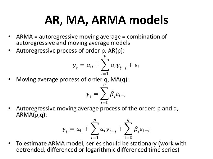
AR, MA, ARMA models •

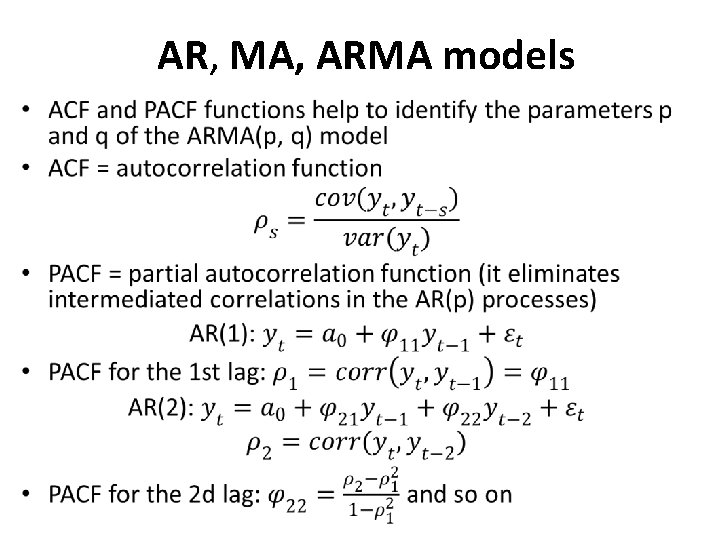
AR, MA, ARMA models •

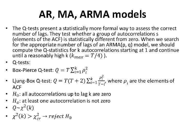
AR, MA, ARMA models •

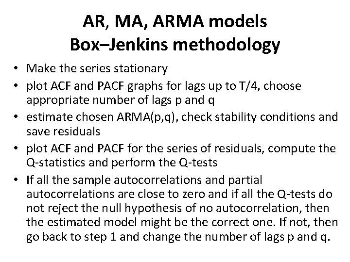
AR, MA, ARMA models Box–Jenkins methodology • Make the series stationary • plot ACF and PACF graphs for lags up to T/4, choose appropriate number of lags p and q • estimate chosen ARMA(p, q), check stability conditions and save residuals • plot ACF and PACF for the series of residuals, compute the Q-statistics and perform the Q-tests • If all the sample autocorrelations and partial autocorrelations are close to zero and if all the Q-tests do not reject the null hypothesis of no autocorrelation, then the estimated model might be the correct one. If not, then go back to step 1 and change the number of lags p and q.

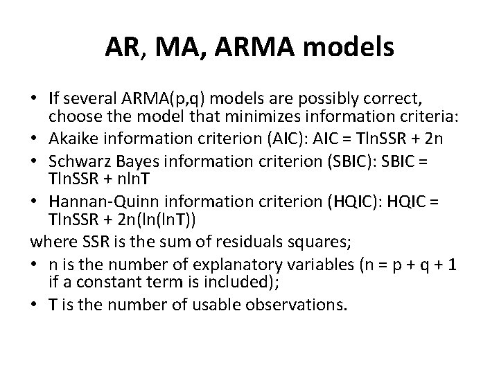
AR, MA, ARMA models • If several ARMA(p, q) models are possibly correct, choose the model that minimizes information criteria: • Akaike information criterion (AIC): AIC = Tln. SSR + 2 n • Schwarz Bayes information criterion (SBIC): SBIC = Tln. SSR + nln. T • Hannan-Quinn information criterion (HQIC): HQIC = Tln. SSR + 2 n(ln(ln. T)) where SSR is the sum of residuals squares; • n is the number of explanatory variables (n = p + q + 1 if a constant term is included); • T is the number of usable observations.

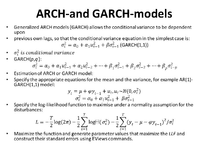
ARCH-and GARCH-models •

ARCH-and GARCH-models •

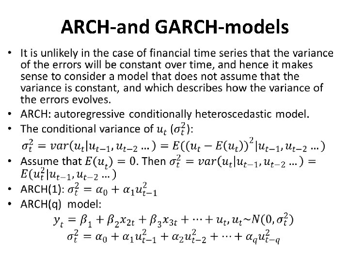
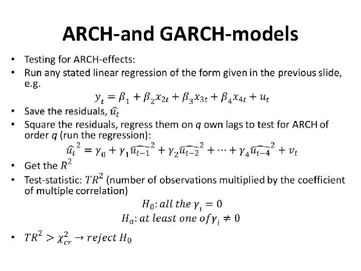
ARCH-and GARCH-models •

Stationarity and unit roots

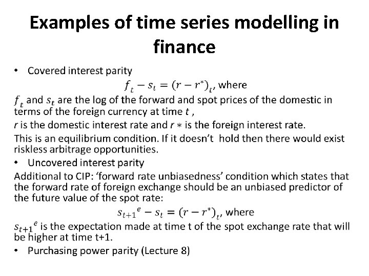
Examples of time series modelling in finance •

Conclusions • We’ve covered how to make the forecast for autoregressive moving average (ARMA) models and exponential smoothing models • How to estimate the accuracy of predictions with the use of different metrics • How to estimate time series models and make the forecasts in EViews

References • Brooks C. Introductory Econometrics for Finance. Cambridge University Press. 2008. • Cuthbertson K. , Nitzsche D. Quantitative Financial Economics. Wiley. 2004. • Tsay R. S. Analysis of Financial Time Series, Wiley, 2005. • Y. Ait-Sahalia, L. P. Hansen. Handbook of Financial Econometrics: Tools and Techniques. Vol. 1, 1 st Edition. 2010. • Alexander C. Market Models: A Guide to Financial Data Analysis. Wiley. 2001. • Cameron A. and Trivedi P. . Microeconometrics. Methods and Applications. 2005. • Lai T. L. , Xing H. Statistical Models and Methods for Financial Markets. Springer. 2008. • Poon S-H. A practical guide forecasting financial market volatility. Wiley, 2005. • Rachev S. T. et al. Financial Econometrics: From Basics to Advanced Modeling Techniques, Wiley, 2007.