Econometric Analysis of Panel Data Random Regressors Pooled

Econometric Analysis of Panel Data • Random Regressors – Pooled (Constant Effects) Model • Instrumental Variables – Fixed Effects Model – Random Effects Model – Hausman-Taylor Estimator

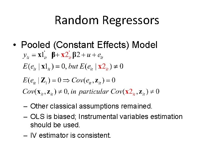
Random Regressors • Pooled (Constant Effects) Model – Other classical assumptions remained. – OLS is biased; Instrumental variables estimation should be used. – IV estimator is consistent.

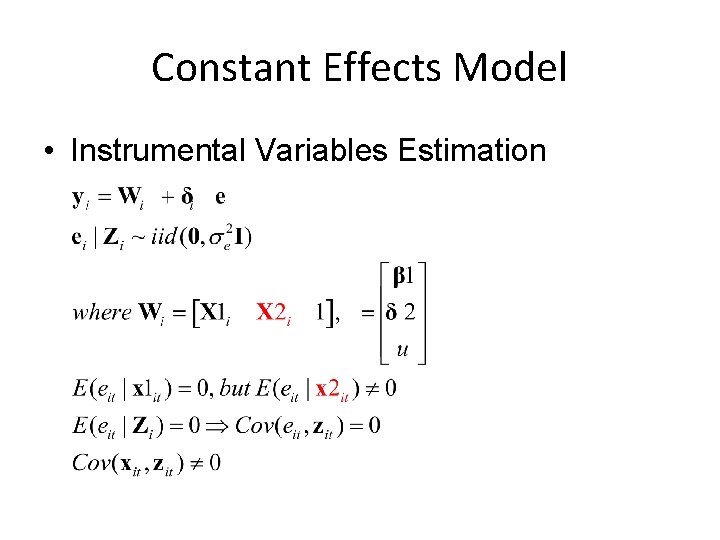
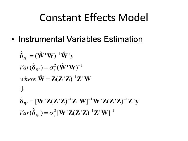
Constant Effects Model • Instrumental Variables Estimation

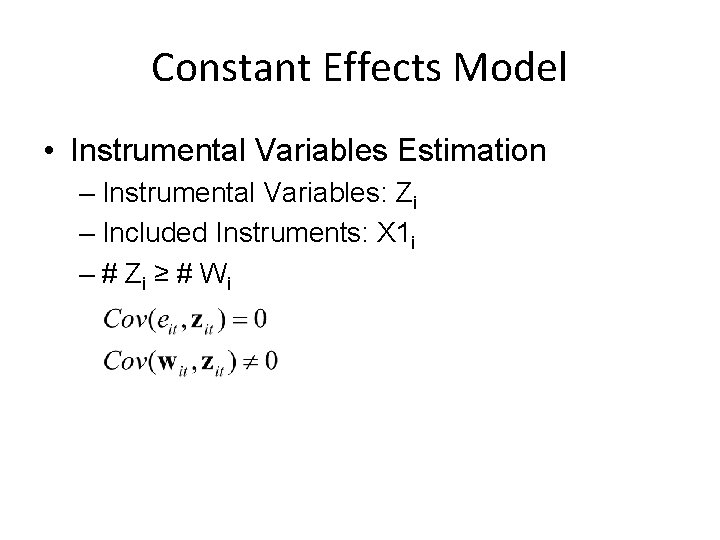
Constant Effects Model • Instrumental Variables Estimation – Instrumental Variables: Zi – Included Instruments: X 1 i – # Zi ≥ # W i

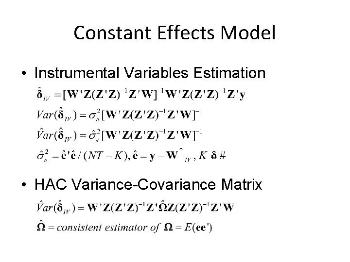
Constant Effects Model • Instrumental Variables Estimation

Constant Effects Model • Instrumental Variables Estimation • HAC Variance-Covariance Matrix

Constant Effects Model • Hypothesis Testing of Instrumental Variables – Test for Endogeneity – Test for Overidentification – Test for Weak Instruments

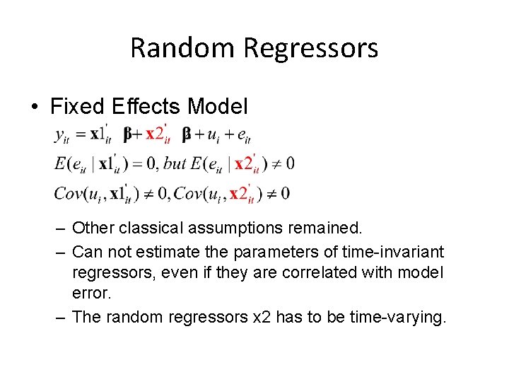
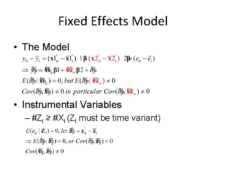
Random Regressors • Fixed Effects Model – Other classical assumptions remained. – Can not estimate the parameters of time-invariant regressors, even if they are correlated with model error. – The random regressors x 2 has to be time-varying.

Fixed Effects Model • The Model • Instrumental Variables – #Zi ≥ #Xi (Zi must be time variant)

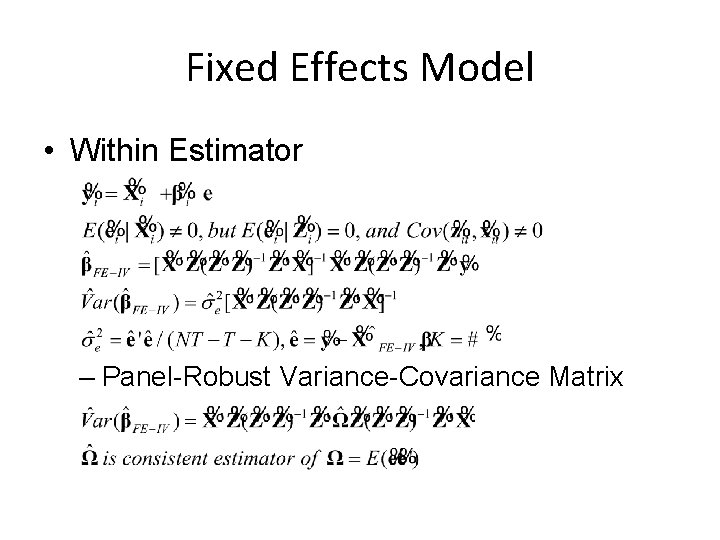
Fixed Effects Model • Within Estimator – Panel-Robust Variance-Covariance Matrix

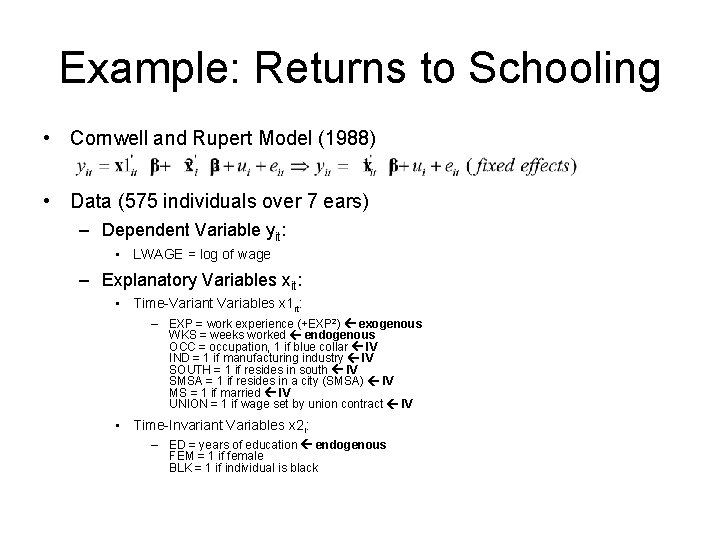
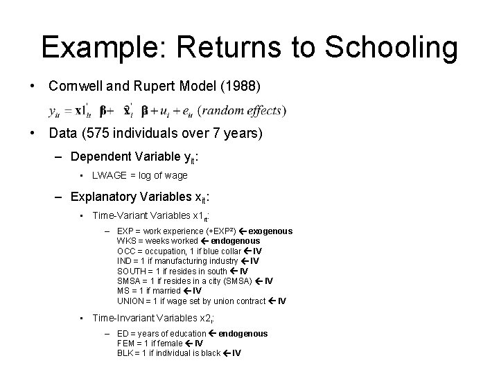
Example: Returns to Schooling • Cornwell and Rupert Model (1988) • Data (575 individuals over 7 ears) – Dependent Variable yit: • LWAGE = log of wage – Explanatory Variables xit: • Time-Variant Variables x 1 it: – EXP = work experience (+EXP 2) exogenous WKS = weeks worked endogenous OCC = occupation, 1 if blue collar IV IND = 1 if manufacturing industry IV SOUTH = 1 if resides in south IV SMSA = 1 if resides in a city (SMSA) IV MS = 1 if married IV UNION = 1 if wage set by union contract IV • Time-Invariant Variables x 2 i: – ED = years of education endogenous FEM = 1 if female BLK = 1 if individual is black

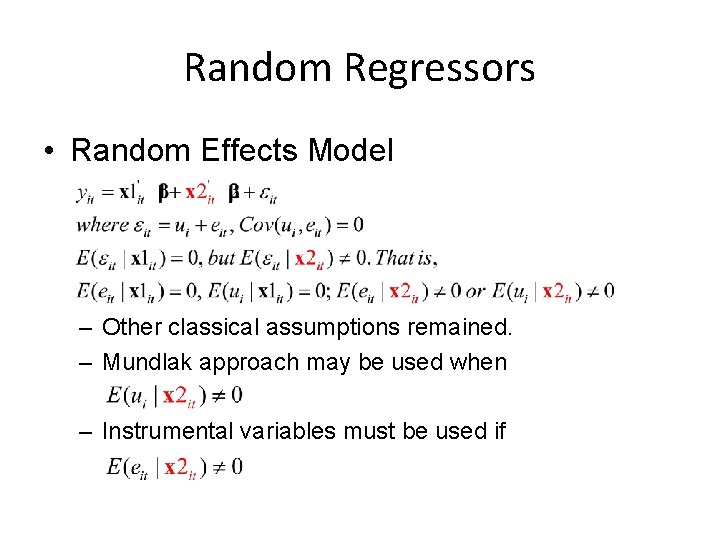
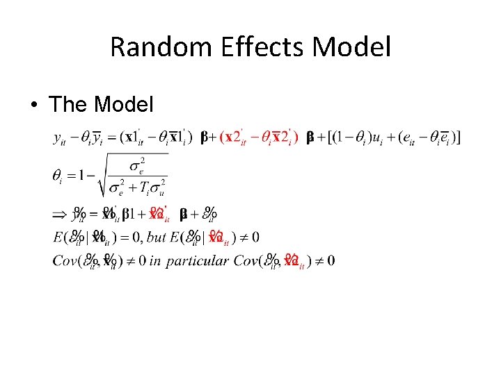
Random Regressors • Random Effects Model – Other classical assumptions remained. – Mundlak approach may be used when – Instrumental variables must be used if

Random Effects Model • The Model

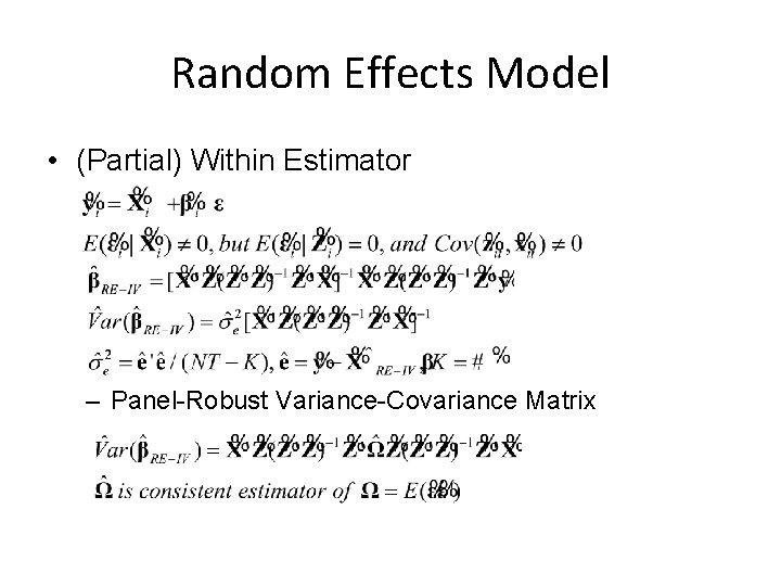
Random Effects Model • (Partial) Within Estimator – Panel-Robust Variance-Covariance Matrix

Example: Returns to Schooling • Cornwell and Rupert Model (1988) • Data (575 individuals over 7 years) – Dependent Variable yit: • LWAGE = log of wage – Explanatory Variables xit: • Time-Variant Variables x 1 it: – EXP = work experience (+EXP 2) exogenous WKS = weeks worked endogenous OCC = occupation, 1 if blue collar IV IND = 1 if manufacturing industry IV SOUTH = 1 if resides in south IV SMSA = 1 if resides in a city (SMSA) IV MS = 1 if married IV UNION = 1 if wage set by union contract IV • Time-Invariant Variables x 2 i: – ED = years of education endogenous FEM = 1 if female IV BLK = 1 if individual is black IV

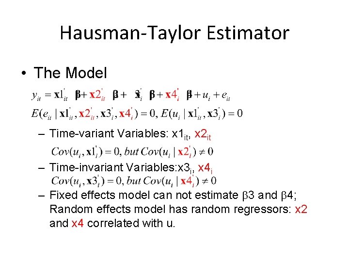
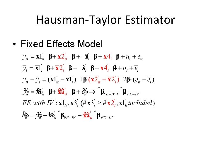
Hausman-Taylor Estimator • The Model – Time-variant Variables: x 1 it, x 2 it – Time-invariant Variables: x 3 i, x 4 i – Fixed effects model can not estimate b 3 and b 4; Random effects model has random regressors: x 2 and x 4 correlated with u.

Hausman-Taylor Estimator • Fixed Effects Model

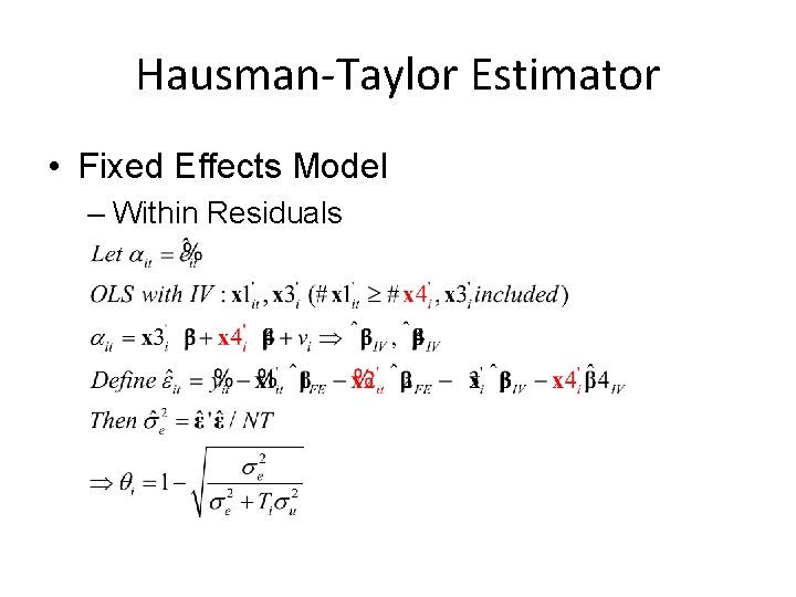
Hausman-Taylor Estimator • Fixed Effects Model – Within Residuals

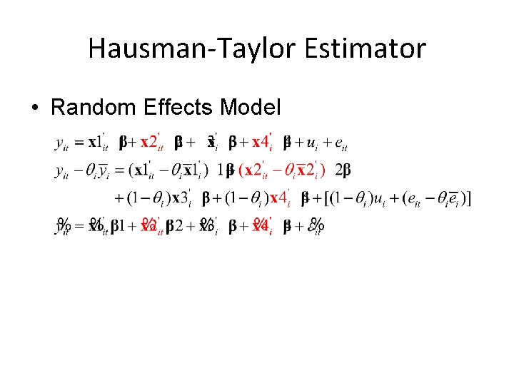
Hausman-Taylor Estimator • Random Effects Model

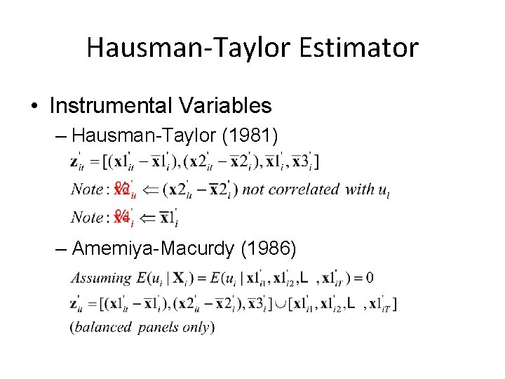
Hausman-Taylor Estimator • Instrumental Variables – Hausman-Taylor (1981) – Amemiya-Macurdy (1986)

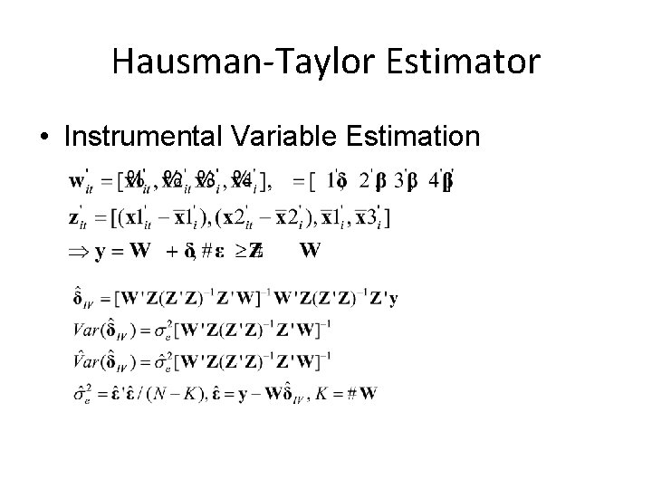
Hausman-Taylor Estimator • Instrumental Variable Estimation

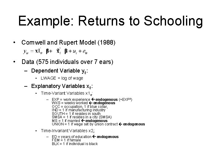
Example: Returns to Schooling • Cornwell and Rupert Model (1988) • Data (575 individuals over 7 ears) – Dependent Variable yit: • LWAGE = log of wage – Explanatory Variables xit: • Time-Variant Variables x 1 it: – EXP = work experience endogenous (+EXP 2) WKS = weeks worked endogenous OCC = occupation, 1 if blue collar, IND = 1 if manufacturing industry SOUTH = 1 if resides in south SMSA = 1 if resides in a city (SMSA) MS = 1 if married endogenous UNION = 1 if wage set by union contract endogenous • Time-Invariant Variables x 2 i: – ED = years of education endogenous FEM = 1 if female BLK = 1 if individual is black