Econometric Analysis of Panel Data Fixed Effects and
![Example: U. S. Productivity • The Model (Munnell [1988]) – Two-level model – Three-level Example: U. S. Productivity • The Model (Munnell [1988]) – Two-level model – Three-level](https://slidetodoc.com/presentation_image_h/f900f43a749be6d0063da119165e553d/image-14.jpg)
- Slides: 16

Econometric Analysis of Panel Data • Fixed Effects and Random Effects: Extensions – Time-invariant Variables – Two-way Effects – Nested Random Effects

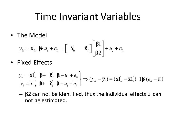
Time Invariant Variables • The Model • Fixed Effects – b 2 can not be identified, thus the individual effects ui can not be estimated.

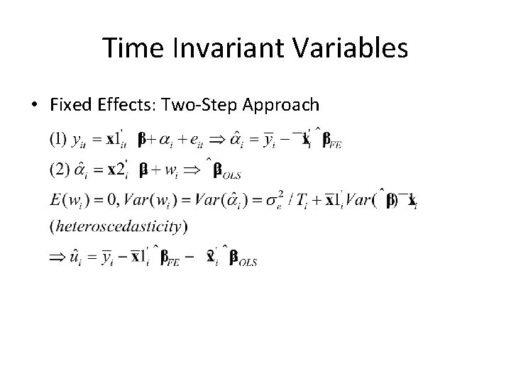
Time Invariant Variables • Fixed Effects: Two-Step Approach

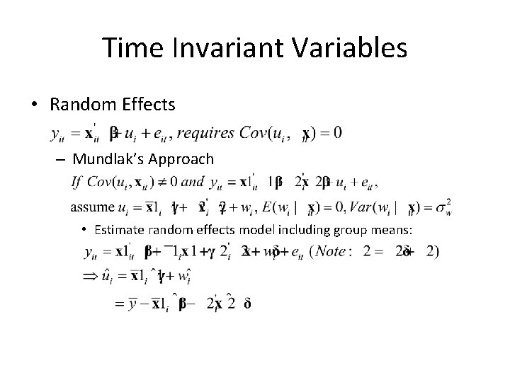
Time Invariant Variables • Random Effects – Mundlak’s Approach • Estimate random effects model including group means:

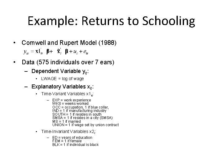
Example: Returns to Schooling • Cornwell and Rupert Model (1988) • Data (575 individuals over 7 ears) – Dependent Variable yit: • LWAGE = log of wage – Explanatory Variables xit: • Time-Variant Variables x 1 it: – EXP = work experience WKS = weeks worked OCC = occupation, 1 if blue collar, IND = 1 if manufacturing industry SOUTH = 1 if resides in south SMSA = 1 if resides in a city (SMSA) MS = 1 if married UNION = 1 if wage set by union contract • Time-Invariant Variables x 2 i: – ED = years of education FEM = 1 if female BLK = 1 if individual is black

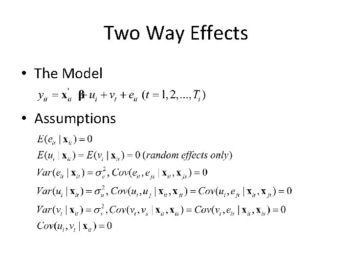
Two Way Effects • The Model • Assumptions

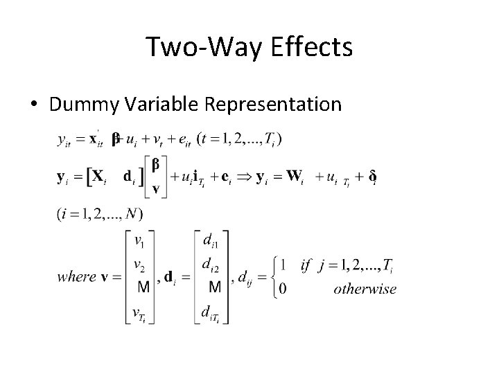
Two-Way Effects • Dummy Variable Representation

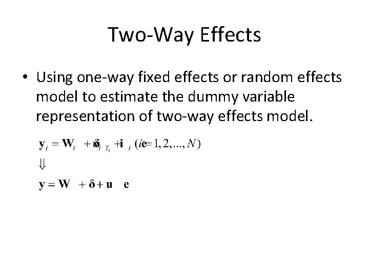
Two-Way Effects • Using one-way fixed effects or random effects model to estimate the dummy variable representation of two-way effects model.

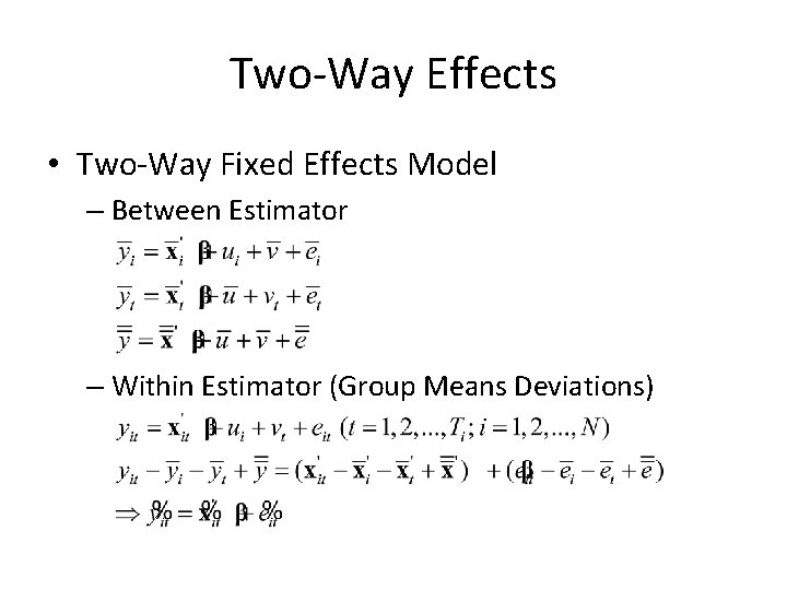
Two-Way Effects • Two-Way Fixed Effects Model – Between Estimator – Within Estimator (Group Means Deviations)

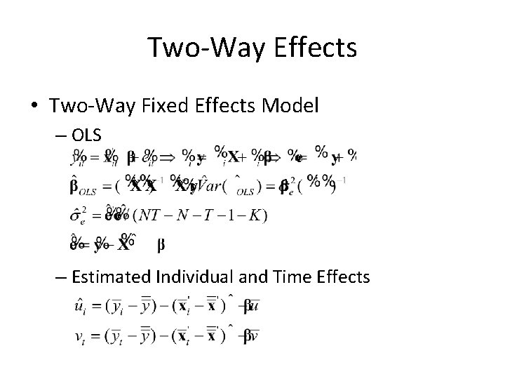
Two-Way Effects • Two-Way Fixed Effects Model – OLS – Estimated Individual and Time Effects

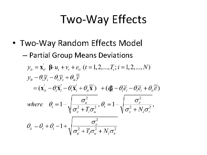
Two-Way Effects • Two-Way Random Effects Model – Partial Group Means Deviations

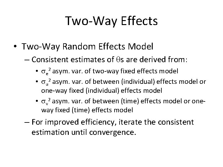
Two-Way Effects • Two-Way Random Effects Model – Consistent estimates of qs are derived from: • se 2 asym. var. of two-way fixed effects model • su 2 asym. var. of between (individual) effects model or one-way fixed (individual) effects model • sv 2 asym. var. of between (time) effects model or oneway fixed (time) effects model – For improved efficiency, iterate the consistent estimation until convergence.

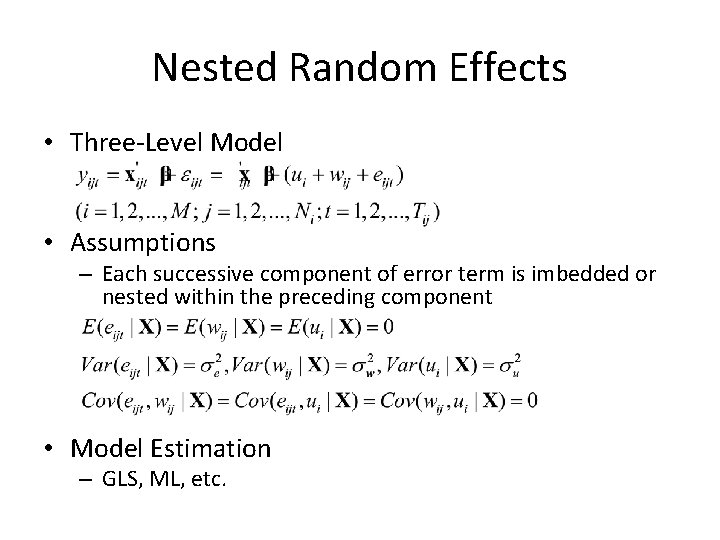
Nested Random Effects • Three-Level Model • Assumptions – Each successive component of error term is imbedded or nested within the preceding component • Model Estimation – GLS, ML, etc.
![Example U S Productivity The Model Munnell 1988 Twolevel model Threelevel Example: U. S. Productivity • The Model (Munnell [1988]) – Two-level model – Three-level](https://slidetodoc.com/presentation_image_h/f900f43a749be6d0063da119165e553d/image-14.jpg)
Example: U. S. Productivity • The Model (Munnell [1988]) – Two-level model – Three-level model – See, B. H. Baltagi, S. H. Song, and B. C. Jung, The Unbalanced Nested Error Component Regression Model, Journal of Econometrics, 101, 2001, 357 -381.

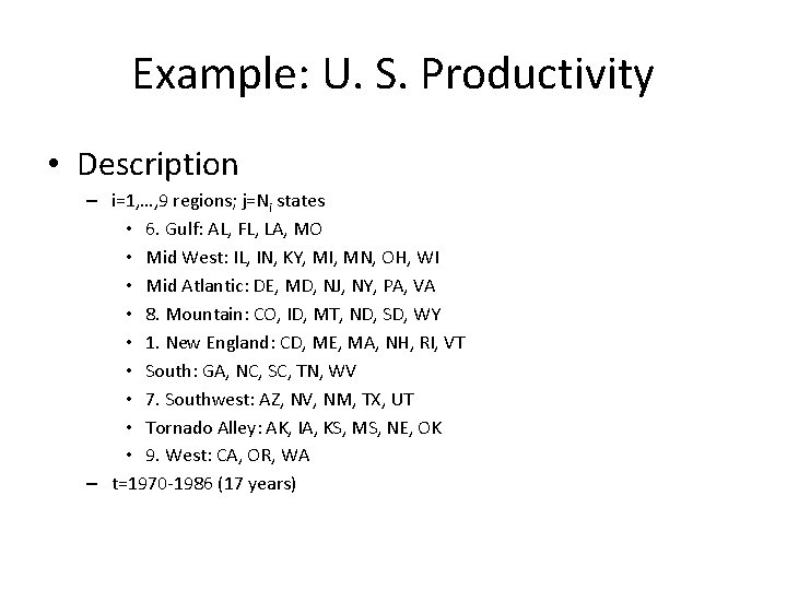
Example: U. S. Productivity • Description – i=1, …, 9 regions; j=Ni states • 6. Gulf: AL, FL, LA, MO • Mid West: IL, IN, KY, MI, MN, OH, WI • Mid Atlantic: DE, MD, NJ, NY, PA, VA • 8. Mountain: CO, ID, MT, ND, SD, WY • 1. New England: CD, ME, MA, NH, RI, VT • South: GA, NC, SC, TN, WV • 7. Southwest: AZ, NV, NM, TX, UT • Tornado Alley: AK, IA, KS, MS, NE, OK • 9. West: CA, OR, WA – t=1970 -1986 (17 years)

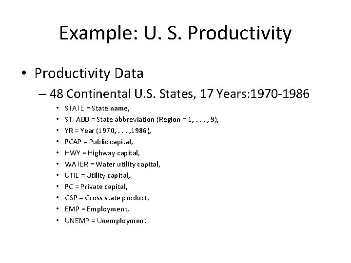
Example: U. S. Productivity • Productivity Data – 48 Continental U. S. States, 17 Years: 1970 -1986 • • • STATE = State name, ST_ABB = State abbreviation (Region = 1, . . . , 9), YR = Year (1970, . . . , 1986), PCAP = Public capital, HWY = Highway capital, WATER = Water utility capital, UTIL = Utility capital, PC = Private capital, GSP = Gross state product, EMP = Employment, UNEMP = Unemployment